NonParametric Superposition example
This example uses the output from the semicompartmental modeling example, detailed in the “Semicompartmental model example”. The study data are from an early Phase I PK/PD trial. Quick input is sought for the design of a seven day multiple dose study. However, the profiles are irregular, and it is not easy to apply a compartmental modeling approach to the data.
This section uses the NonParametric Superposition object to predict plasma concentrations and effect-site concentrations at steady-state based on single-dose data. This feature allows for predictions on data that are otherwise difficult to model.
Knowledge of how to do basic tasks using the Phoenix interface, such as creating a project and importing data, is assumed.
The completed project (NPS.phxproj) is available for reference in …\Examples\WinNonlin.
Set up an estimation of steady-state plasma concentrations
Create a project called NPS.
Import the files …\Examples\WinNonlin\Supporting files\SCM_Results.xls.
In the File Import Wizard dialog, select the Has units row option.
Right-click SCM_Results in the Data folder and select Send To > NonCompartmental Analysis > NonParametric Superposition.
In the Main Mappings panel, map the columns to the contexts as follows:
Subject to Sort.
Conc to Concentration.
Leave Time mapped to Time.
Leave Ce mapped to None.
Leave Effect mapped to None.
In the Options tab below the Setup panel, type 50 in the Loading Dose field.
In the Maintenance Dose field type 50.
In the Tau (dosing interval) field type 4.
Execute and view the plasma estimation results
1. Click ![]() (Execute icon) to execute the object.
(Execute icon) to execute the object.
The Concentration worksheet provide predicted steady-state plasma concentrations. The Lambda z worksheet lists the Lambda Z and half-life estimates.

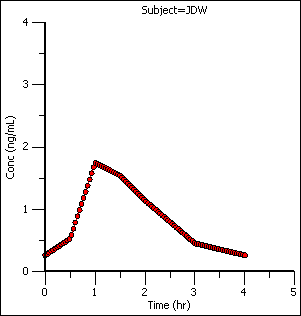
The plot output shows predicted steady state concentrations over time for each subject. The first subject’s plot is shown below.

Set up an estimation of steady-state effect-site concentrations
1. Select the NonParametric object’s Setup panel.
2. In the Main Mappings panel, re-map the columns to the contexts as follows:
Conc to None.
Ce to Concentration.
Leave Subject mapped to Sort.
Leave Time mapped to Time.
Leave Effect mapped to None.
3. Select Terminal Phase from the Setup list.
4. Check the Use Internal Worksheet box.
5. For each row:
a. In the Start column, type 4.
b. In the End column, type 8.
Execute and view the effect-site concentration estimation results
1. Execute the object.
The new NonParametric worksheet results provide predicted effect site concentrations at steady-state and Lambda Z and half-life estimates.

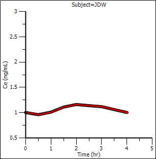
The plot output shows predicted effect site concentrations at steady-state over time for each subject. The first subject’s graph is shown below.

Compute the steady-state effect
Now it is possible to compute the steady-state effect from the predicted steady-state concentrations at the effect site.
In the Semicompartmental example, the PD model 103 was used (its sample graph is shown below). The effect formula for model 103 is E=E0*(1 – (C/(C+IC50))). This formula will be adjusted for each subject in the study.

1. In the Results tab, right-click the Concentrations (effect site concentrations) worksheet and select Copy to Data Folder.
The worksheet is added to the project’s Data folder and renamed “Concentrations from NonParametric”.
2. In the Object Browser, select Concentrations from NonParametric in the Data folder.
3. In the Columns tab below the table, press Add under the Columns list.
4. In the New Column Properties dialog, the Numeric option button is selected by default. Do not change this setting.
5. In the Column Name field type Effect and press OK.
The Effect column is added in the Columns list and in the table in the Grid tab.
6. Use the Down Arrow button beside the Columns list to move the Effect column header to the bottom of the Columns list.
7. In the Object Browser, right-click Concentrations from NonParametric and select Edit in Excel.
Phoenix displays a message warning that changes made in Excel are not recorded in Phoenix.
8. Press OK.
The worksheet is opened in Excel. If you see a pop-up dialog stating that the format and extension of the file do not match, press Yes to continue as the file is safe to open.
In Excel, enter the PD model 103 effect formula in the Effect column for each subject at time zero. Use the E0 and IC50 values from the PD Model object’s Final Parameters worksheet.
9. Select the cell in the Effect column at time zero for the first subject, JDW.
10. Type the effect formula shown below in the Effect column cell at time 0 (zero) for subject JDW, which is row 3.
= 102.93*(1-(C3/(C3+0.09))) (for subject JDW)
11. Repeat for the second and third subjects, LEJ (row 104) and SCC (row 205).
= 100.17*(1-(C104/(C104+0.09))) (for subject LEJ)
= 100.45*(1-(C205/(C205+0.08))) (for subject SCC)
12. After the Effect value formula is set up at time zero for each subject copy the formula to the other time points for each subject.
Because of the way Phoenix handles its interactions with Excel, the Save As option in Excel cannot be used to save the worksheet with a different name or to a different location. The Save option must be used.
13. Select File > Save.
14. Close Excel. Be sure to save the worksheet before closing Excel, or all changes are lost.
An Apply Changes message dialog is displayed.
15. Press Yes to apply the changes. An entry is written in the worksheet History tab noting that it was edited in Excel.
16. When asked whether to save formulas, select No so that the worksheet is editable in Phoenix.
The Concentrations from NonParametric worksheet now has Effect values derived from the equations used in the Excel edit and can still be used with operational objects.
Plot time vs effect
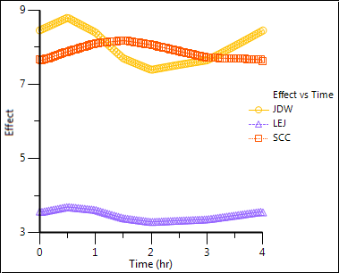
Once the steady-state effects and concentrations are generated it is possible to use the modified concentrations from NonParametric worksheet to plot time vs. effect for each subject by mapping the worksheet to an XY Plot object.
1. Right-click Concentrations from NonParametric in the Data folder and select Send To > Plotting > XY Plot.
2. In the XY Data Mappings panel, map the columns to the contexts as follows:
Subject to Group.
Time to X.
Effect to Y.
Leave Ce mapped to None.
3. Execute the object.

This concludes the Nonparametric superposition example.