Variations in models using Phenobarbital data
The data in pheno.dat come from a study of the neonatal pharmacokinetics of phenobarbital reported by Grasela and Donn. (Grasela and Donn (1985). Neonatal Population Pharmacokinetics of Phenobarbital Derived from Routine Clinical Data. Dev Pharmacol Ther, 8:372–383.).
Data were collected on 59 pre-term infants given phenobarbital for prevention of seizures during the first 16 days after birth. Each individual received an initial dose followed by one or more sustaining doses by intravenous administration. A total of between one and six concentration measurements were obtained from each individual at times other than dose times as part of routine monitoring, for a total of 155 measurements. Additionally, birth weight (wt) and a five-minute Apgar score (Apgar < 5) were recorded for each subject.
The pharmacokinetics of phenobarbital can be described by a one-compartment model with intravenous administration and first-order elimination, which is found in Phoenix library models as PK model 1. In this model, the subject-specific pharmacokinetic parameters to be estimated are the elimination rate constant, Ke, and volume of distribution, V.
Note: The completed project (Pheno.phxproj) is available for reference in …\Examples\NLME.
Set up the Maximum Likelihood Models object
Create a new project called Pheno.
Import the dataset …\Examples\NLME\Supporting files\pheno.dat.
Press Finish in the File Import Wizard dialog.
Right-click Workflow and select New > Modeling > Maximum Likelihood Models.
Rename the Maximum Likelihood Models object Pheno Model.
Select the Parameters > Structural sub-tab.
Press Add Covariate.
Type wt in the Covariate field. wt is added as a context association in the Main Mappings panel.
Press Add Covariate.
Type apgr in the Covariate field. apgr is added as a context association in the Main Mappings panel.
Note: Adding weight (wt) and Apgar (apgr) as covariates allows Phoenix to create covariate plots in the output.
Map the pheno dataset
1. Drag the pheno worksheet from the Data folder to the Main Mappings panel.
2. Map the columns to the contexts as follows:
xid to ID.
time to Time.
dose to A1.
wt to wt.
apgr to apgr.
yobs to CObs.
Leave idum1 mapped to None.
Leave idum2 mapped to None.
3. In the Structure tab, select Micro from the Parameterization menu.
4. Select the Run Options tab.
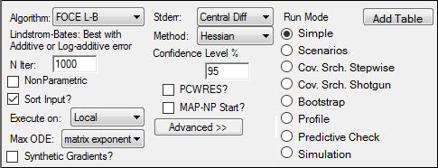
5. Select FOCE L-B as the Algorithm and Hessian as the Method.

6. Click ![]() (Execute icon) to execute the object.
(Execute icon) to execute the object.
Set up the full block model
1. Right-click Pheno Model and select Copy.
2. Right-click Workflow and select Paste.
3. Rename the project as Pheno Block.
The columns are automatically mapped as follows:
xid to ID.
time to Time.
dose to A1.
wt to wt.
apgr to apgr.
yobs to CObs.
idum1 mapped to None.
idum2 mapped to None.
4. Select the Parameters > Fixed Effects sub-tab.
5. Press Accept All Fixed+Random to copy the new estimates to the Initial estimates field for each parameter.
6. Select the Random Effects sub-tab.
7. Clear the Diag checkbox to use the full block structure.
8. Execute the object.
Add covariate effects to study parameters
1. Right-click Pheno Block and select Copy.
2. Right-click Workflow and select Paste.
3. Rename the project as Pheno Block Covar.
4. Select the Parameters > Fixed Effects sub-tab.
5. Press Accept All Fixed+Random to copy the new estimates to the Initial estimates field for each parameter.
6. Select the Structural sub-tab.
7. Underneath the V parameter, click No for the wt covariate to change it to Yes.
8. Underneath the Ke parameter, click No for the wt covariate to change it to Yes.
The study variable wt is added as a covariate effect to both V and Ke.
9. Underneath the V parameter, click No for the apgr covariate to change it to Yes.
The study variable apgr is added as a covariate effect to V.

The columns are automatically mapped as follows:
xid to ID.
time to Time.
dose to A1.
wt to wt.
apgr to apgr.
yobs to CObs.
idum1 mapped to None.
idum2 mapped to None.
10. Execute the object.
Save and close the project
1. Select File > Save Project.
2. Press Save.
3. Select File > Close Project.
The project is saved and closed and Phoenix can be safely closed.
This concludes the model variations example that uses Phenobarbital data.