Simple PK population analysis using QRPEM
This example shows how to perform a simple PK population analysis with the QRPEM engine, including dataset importation, model set up, and execution for a simple one-compartment model with parameter Cl (Clearance) and V (Volume).
Data and dosing information are assumed already collected for each patient and entered in a data file (model1pkcl.csv).
Also assumed available, using either prior information or tools like non-compartmental analysis or graphical tools in Phoenix, are initial values for the population mean of Cl and V. These will be needed by the model.
Note: The completed project (1c_iv_qrpem.phxproj) is available for reference in …\Examples\NLME.
Set up the Maximum Likelihood Models object
Create a new project called 1c_iv_qrpem.
Import the dataset …\Examples\NLME\Supporting files\model1pkcl.csv.
Press Finish in the File Import Wizard dialog.
Right-click the worksheet and select Send To > Modeling > Maximum Likelihood Models.
In the Main Mappings panel, map the columns to the contexts as follows:
AMT to A1.
DV to CObs.
ID and Time are automatically mapped.
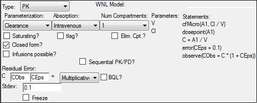
In the Structure tab, make sure the Parameterization menu is set to Clearance, the Absorption menu to Intravenous, and the Num menu to 1.
Set the Residual Error menu to Multiplicative.
Keep the Stdev value of 0.1.

Note: For PK data with an assumed proportional error model, the use of 0.1 (10% error) as initial input for the standard deviation is often reasonable. Since sigma is also optimized, any prior knowledge is beneficial and can prevent potential confounding between the within (sigma) and between (Omega) subject variability model-based parameters.
Enter initial estimates for the population means
The MCPEM/QRPEM algorithm’s first step requires an initial estimate for the population mean (Fixed Effect) and variance (Random Effect). For each patient, given its data, Phoenix NLME will take these population means and variance (and Sigma) as input and will estimate the set of parameters that explain the patient’s response data. The algorithm finds the sets of values that could explain the same data and, since each set has a different probability in explaining the patient’s data, it defines a distribution (referred to as a posterior distribution).
1. Select the Parameters > Fixed Effects sub-tab.
2. Enter the following initial estimates:
tvV = 50
tvCl = 5
3. Select the Random Effects sub-tab.
4. Clear the Diag checkbox to specify a full variance covariance matrix.
5. Enter 1 for all diagonal entries and 0 for off-diagonal.
Starting with initial estimates for the mean and variance and the number of samples to estimate for each patient, the algorithm estimates the individual posterior distributions for each patient. This is used as the sample at the first iteration.
The algorithm then updates the mean and population variances and generates new posterior distributions which are used as the new sample for each patient. The iterations continue, using the same algorithm but with new mean, variances, and sigma.
Usually, 50 iterations are enough to reach convergence (i.e., no noticeable change in the means, variances, sigma, and log-likelihood). Since the algorithm uses samples, there may be small oscillations in the log-likelihood but no increasing or decreasing trend once convergence is reached.
6. Select the Run Options tab.
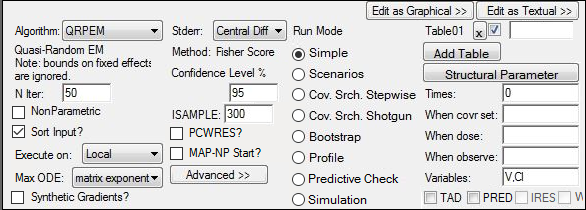
7. From the Algorithm menu, select QRPEM.
8. Enter 50 iterations for N iter.
To obtain the best model parameters for each patient, add a table.
9. Press Add Table.
10. Enter 0 for Times.
11. Press the Structural Parameter button to list the structural parameters in the Variables field.

12. Click ![]() (Execute icon).
(Execute icon).
13. In the Results tab, click Table01 under Output Data.
Table01 reports the individual Cl and V values for each patient (the mode of each individual posterior distribution).
14. Click Theta and Omega under Output Data.
The final estimates for fixed effects and sigma can be found in the Theta table. The final estimates for the covariance matrix of random effects can be found in the Omega table.
Use the MAP
So far in this example, the default method has been used. This method works well when data is not too rich. The main settings used for the default algorithm include 300 samples for each patient, perform a MAP estimation only at the first iteration, and do a maximum of 50 iterations.
When data is rich, each patient will be defined by very few Cl and V value sets, with most of the weight on only one set of model parameters. With very rich data, the program can have problems with the default algorithm as the individual posterior variances collapse easily to zero because there are not enough random samples and because the true posterior variances are small. When this happens, the estimated posterior variances from iteration two can collapse and it is better to ask the program to do a MAP estimation at each iteration. Increasing the number of samples should also be done.
1. In the Object Browser, right-click ML Model and select Copy.
2. Right-click Workflow and select Paste.
3. Rename the copied object as MAP.
4. Select the Run Options tab.
5. Enter 1000 in the ISAMPLE field.
6. Press Advanced >>.
7. Turn on the MAP Assist checkbox.
8. Execute the object.
For comparison, run the model using the FOCE ELS and FOCE L-B engines instead of QRPEM. QRPEM has a more efficient sampling algorithm, so the number of samples will need to be increased.
This concludes the simple PK population analysis using QRPEM example.