A contrast is a linear combination of the parameters associated with a term where the coefficients sum to zero. Contrasts facilitate the testing of linear combinations of parameters. For example, consider a completely randomized design with four treatment groups: Placebo, Low Dose, Medium Dose, and High Dose. It is possible to test the hypothesis that the average of the dosed groups is the same as the average of the placebo group. One could write this hypothesis as:

or, equivalently:

Both of these are contrasts since the sum of the coefficients is zero. Note that both contrasts make the same statement. This is true generally: contrasts are invariant under changes in scaling.
Contrasts are tested using the Wald (1943) test statistic:

where:
 is the estimator of b.
 is the estimator of V.
L must be a matrix such that each row is in the row space of X.
This requirement is enforced in the wizard. The Wald statistic is compared to an F distribution with rank(L) numerator degrees of freedom and denominator degrees of freedom estimated by the program or user-specified.
Joint contrasts are constructed when the number of columns for contrast is changed from the default value of one to a number larger than one. Note that this number must be no more than one less than the number of distinct levels for the model term of interest. This tests both hypotheses jointly, i.e., in a single test with a predetermined level of the test.
A second approach would be to put the same term in the neighboring contrast, both of which have one column. This approach will produce two independent tests, each of which is at the specified level.
To see the difference, compare Placebo to Low Dose and Placebo to Medium Dose. Using the first approach, enter the coefficients as follows.
Title = Join tests
Effect = Treatment
Contrast = Treatment
#1 Placebo –1 –1
#2 Low Dose 1 0
#3 Medium Dose 0 1
#4 High Dose 0 0
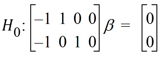
This will produce one test, testing the following hypothesis.

Now compare this with putting the second contrast in its own contrast.
Contrast #1
Title Low vs. Placebo
Effect Treatment
Contrast Treatment
#1 Placebo –1
#2 Low Dose 1
#3 Medium Dose 0
#4 High Dose 0
Contrast #2
Title Medium vs. Placebo
Effect Treatment
Contrast Treatment
#1 Placebo –1
#2 Low Dose 0
#3 Medium Dose 1
#4 High Dose 0
This produces two tests:

Note that this method inflates the overall Type I error rate to approximately 2a, whereas the joint test maintains the overall Type I error rate to a, at the possible expense of some power.
If a contrast is not estimable, then an estimable function will be substituted for the nonestimable function. See the “Substitution of estimable functions for non-estimable functions” section for the details.
The User specified degrees of freedom checkbox available on the Contrasts, Estimates, and Least Squares Means tabs, allows control of the denominator degrees of freedom in the F approximation. The numerator degrees of freedom is always calculated as rank(L). If the checkbox is not selected, then the default denominator degrees of freedom will be used. The default calculation method of the degrees of freedom is controlled on the General Options tab and is initially set to Satterthwaite.
Note: For a purely fixed effects model, Satterthwaite and residual degrees of freedom yield the same number. For details of the Satterthwaite approximation, see the “Satterthwaite approximation for degrees of freedom” section.
To override the default degrees of freedom, select the checkbox and type an appropriate number in the field. The degrees of freedom must greater than zero.
To control the estimability tolerance, enter an appropriate tolerance in the Estimability Tolerance field. For more information see the “Substitution of estimable functions for non-estimable functions” section.
The Show Coefficients checkbox produces extra output, including the coefficients used to construct the tolerance. If the contrast entered is estimable, then it will repeat the contrasts entered. If the contrasts are not estimable, it will enter the estimable function used instead of the nonestimable function.