Modeling and nonlinear regression
Model fitting algorithms and features of Phoenix WinNonlin
Modeling and nonlinear regression
The value of mathematical models is well recognized in all of the sciences — physical, biological, behavioral, and others. Models are used in the quantitative analysis of all types of observations or data, and with the power and availability of computers, mathematical models provide convenient and powerful ways of looking at data. Models can be used to help interpret data, to test hypotheses, and to predict future results. The main concern here is with “fitting” models to data — that is, finding a mathematical equation and a set of parameter values such that values predicted by the model are in some sense “close” to the observed values.
Most scientists have been exposed to linear models, models in which the dependent variable can be expressed as the sum of products of the independent variables and parameters. The simplest example is the equation of a line (simple linear regression):

where Y is the dependent variable, X is the independent variable, A is the intercept and B is the slope. Two other common examples are polynomials such as:

and multiple linear regression.

These examples are all “linear models” since the parameters appear only as coefficients of the independent variables.
In nonlinear models, at least one of the parameters appears as other than a coefficient. A simple example is the decay curve:

This model can be linearized by taking the logarithm of both sides but, as written, it is nonlinear.
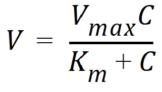
Another example is the Michaelis-Menten equation:

This example can also be linearized by writing it in terms of the inverses of V and C but better estimates are obtained if the nonlinear form is used to model the observations (Endrenyi, ed. (1981), pages 304–305).
There are many models which cannot be made linear by transformation. One such model is the sum of two or more exponentials, such as:

All of the models on this page are called nonlinear models, or nonlinear regression models. Two good references for the topic of general nonlinear modeling are Draper and Smith (1981) and Beck and Arnold (1977). The books by Bard (1974), Ratkowsky (1983) and Bates and Watts (1988) give a more detailed discussion of the theory of nonlinear regression modeling. Modeling in the context of kinetic analysis and pharmacokinetics is discussed in Endrenyi, ed. (1981) and Gabrielsson and Weiner (2016).
All pharmacokinetic models derive from a set of basic differential equations. When the basic differential equations can be integrated to algebraic equations, it is most efficient to fit the data to the integrated equations. But it is also possible to fit data to the differential equations by numerical integration. Phoenix WinNonlin can be used to fit models defined in terms of algebraic equations and models defined in terms of differential equations as well as a combination of the two types of equations.
Given a model of the data, and a set of data, how is the model “fit” to the data? Some criterion of “best fit” is needed, and many have been suggested but only two are much used. These are maximum likelihood and least squares. With certain assumptions about the error structure of the data (no random effects), the two are equivalent. A discussion of using nonlinear least squares to obtain maximum likelihood estimates can be found in Jennrich and Moore (1975). In least squares fitting, the “best” estimates are those which minimize the sum of the squared deviations between the observed values and the values predicted by the model.
The sum of squared deviations can be written in terms of the observations and the model. In the case of linear models, it is easy to compute the least squares estimates. One equates to zero the partial derivatives of the sum of squares with respect to the parameters. This gives a set of linear equations with the estimates as unknowns; well-known techniques can be used to solve these linear equations for the parameter estimates.
This method will not work for nonlinear models, because the system of equations which results by setting the partial derivatives to zero is a system of nonlinear equations for which there are no general methods for solving. Consequently, any method for computing the least squares estimates in a nonlinear model must be an iterative procedure. That is, initial estimates of the parameters are made and then, in some way, these initial estimates are modified to give better estimates, i.e., estimates which result in a smaller sum of squared deviations. The iteration continues until hopefully the minimum (or least) sum of squares is reached.
In the case of models with random effects, such as population PK/PD models, the more general method of maximum likelihood (ML) must be employed. In ML, the likelihood of the data is maximized with respect to the model parameters. The LinMix operational object fits models of this variety.
Since it is not possible to know exactly what the minimum is, some stopping rule must be given at which point it is assumed that the method has converged to the minimum sum of squares. A more complete discussion of the theory underlying nonlinear regression can be found in the books cited previously.