Knowledge of how to do basic tasks using the Phoenix interface, such as creating a project and importing data, is assumed.
The examples project Model_Examples.phxproj located in …\Examples\WinNonlin involve Least-Squares Regression modeling objects. Each model object within this project contains the appropriate default mappings and settings needed to run the model.
To run these example objects:
Load the project …\Examples\WinNonlin\Model_Examples.phxproj into Phoenix.
Each example model has the following items associated with it:
A dataset in workbook form.
Many have datasets in workbook form for dosing.
A PK, PKPD, Indirect Response, or User ASCII model object.
Explore each model object and its mappings and settings.
Execute each model.
Explanations for each model object in the example is given below.
Pharmacokinetic model (Exp1)
In the Exp1 example, a dataset was fit to PK model 13 in the pharmacokinetic model library. Four constants are required for model 13: the stripping dose associated with the parameter estimates, the number of doses, the dose, and the time of dosing.
This example uses weighted least squares (1/observed Y). Phoenix determines initial estimates via curve stripping and then generates bounds for the parameters.
Pharmacokinetic model with multiple doses (Exp2)
In the Exp2 example, a dataset obtained following multiple dosing is fit to model 13 in the pharmacokinetic model library, which is a two-compartment open model. This model has five parameters: A, B, K01, Alpha, and Beta and uses the user-supplied initial values 20, 5, 3, 2, and 0.05. Phoenix generates bounds for the parameters.
Probit analysis: maximum likelihood estimation of potency (Exp3)
The Exp3 example demonstrates how to use the NORMIT and WTNORM functions to perform a probit regression (parallel line bioassay or quantal bioassay) analysis. Note that a probit is a normit plus five. There are several interesting features used in this example:
The transform capability was used to create the response variable.
The logarithm of the relative potency is estimated as a secondary parameter.
Maximum likelihood estimates were obtained by iteratively reweighting and turning off the halvings and convergence criteria. Therefore, instead of iterating until the residual sum of squares is minimized, the program adjusts the parameters until the partial derivatives with respect to the parameters in the model are zero. This will normally occur after a few iterations.
Since there is no s2 in a problem such as this, variances for the maximum likelihood estimates are obtained by setting S2=1 (MEANSQUARE=1).
The following modeling options are used:
Method 3 is selected, which is recommended for Maximum Likelihood estimation (MLE), and iterative reweighting problems.
Convergence Criterion is set to 0. This turns off convergence checks for MLE.
Iterations are set to 10. Estimates should converge after a few iterations.
Meansquare is set to 1. Sigma squared is 1 for MLE.
For further reading regarding use of nonlinear least squares to obtain maximum likelihood estimates, refer to Jennrich and Moore (1975). Maximum likelihood estimation by means of nonlinear least squares. Amer Stat Assoc Proceedings Statistical Computing Section 57–65.
Logit regression (bioassay) (Exp4)
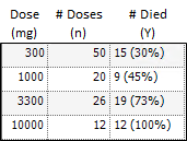
The following data were obtained in a toxicological experiment:

In the Exp4 example, assume that the distribution of Y is binomial with:
mean = np
variance = npq, and q=1 – p
where:

and X = loge dose
Maximum likelihood estimates of a and b for this model are obtained via iteratively reweighted least squares. This is done by fitting the mean function (np) to the Y data with weight (npq) –1.
The modeling commands needed to fit this model to the data are included in an ASCII model file. Note that the loge LD50 and loge LD001 are also estimated as secondary parameters.
This model is really a linear logit model in that:

Note: For this type of problem, the final value of the residual sum of squares is the Chi-square statistic for testing heterogeneity of the model. If this example is executed, X2 (heterogeneity) = 2.02957, with 4 – 2 = 2 degrees of freedom (number of data points minus the number of parameters that were estimated).
For a more in-depth discussion of the use of nonlinear least squares for maximum likelihood estimation, see Jennrich and Moore (1975). Maximum likelihood estimation by means of nonlinear least squares. Amer Stat Assoc Proceedings Statistical Computing Section 57–65.
In the Engine Settings tab, the Convergence Criteria is set to zero to turn off the halving and convergence checks. Meansquare is set to 1 (the residual mean square is redefined to be 1.00) in order to estimate the standard errors of a, b, and the secondary parameters.
Survival analysis (Exp5)
Exp5 is another maximum likelihood example and is very similar to Model Exp4. It is included to show that models arising in a variety of disciplines, such as case survival or reliability analysis, can be fit by nonlinear least squares.
The dosing constant is defined in this model as the denominator for the proportions, that is, N.
In the Engine Settings tab the Convergence Criteria is set to zero to turn off the halving and convergence checks. Meansquare is set to 1 (redefines the residual mean square to be 1.00) in order to estimate the standard errors of the primary and secondary parameters.
Two differential equations with data for both compartments (Exp6)
Exp6 involves the following model:

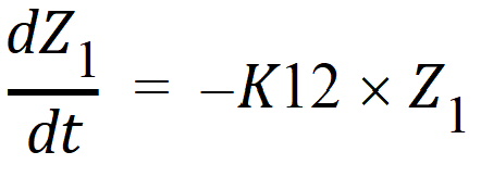
where K12 and K20 are first-order rate constants. This model may be described by the following system of two differential equations.
 compartment 1
 compartment 2
with initial conditions Z1=D, and Z2=0.
In addition to obtaining estimates of K12 and K20, it is also desirable to estimate D and the half-lives of K12 and K20.
A sample solution for this example is given here. Note that, for this example, the model is defined as an ASCII file. Data corresponding to both compartments are available.
Column C in the dataset for this example contains a function variable, which defines the separate functions.
Two differential equations with data on one-compartment (Ex7)
The model for the Exp7 example is identical to that for Exp6. However, in this example, it is assumed that data are available only for compartment two.
Multiple linear regression (Exp8)
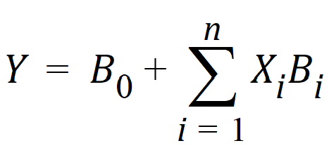
Linear regression models are a subset of nonlinear regression models; consequently, linear models can also be fit using Phoenix. To illustrate this, a sample dataset (taken from Analyzing Experimental Data By Regression by Allen and Cady (1982), Lifetime Learning Publications, Belmont, CA) was analyzed in Exp8. Note that linear models can always be written as:

This example is also interesting in that the model was initially defined in such a way to permit several different models to be fit to the data.
In the ASCII model panel, note that the number of parameters to be estimated is defined in CONS in order to make the model specification as general as possible. Note also the use of a DO loop in the model text.
Note: When using Phoenix to fit a linear regression model:
- use arbitrary initial values
- make sure the Do Not Use Bounds option is checked
- select the Gauss-Newton minimization method with the Levenberg and Hartley modification
The dosing constant for this example is the number of terms to be fit in the regression.
Cumulative areas under the curve (Exp9)
The Exp9 example uses the TRANSFORM block of commands to output cumulative area under the curve values calculated by trapezoidal rule. It computes cumulative urine excretion then fits it to a one-compartment model. The use of the LAG function is demonstrated.
Mitscherlich nonlinear model (Exp10)
In the Exp10 example, a dataset is fit to the Mitscherlich model. The data were taken from Allen and Cady (1982), Analyzing Experimental Data By Regression. Lifetime Learning Publications, Belmont, CA. Fitting data to this model involves the estimation of three parameters; b1, b2, and a.

Four parameter logistic model (Exp11)
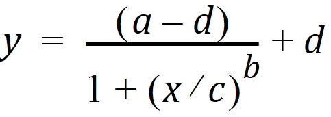
The Exp11 example illustrates how to fit a dataset to a general four parameter logistic function. The function is often used to fit radioimmunoassay data. The function, when graphed, depicts a sigmoidal (S-shaped) curve. The four parameters represent the lower and upper asymptotes, the ED50, and a measure of the steepness of the slope. For further details see DeLean, Munson and Rodbard (1978). Simultaneous analysis of families of sigmoidal curves: Application to bioassay, radioligand assay and physiological dose-response curves. Am J Physiol 235(2):E97–E102. The model, with parameters a, b, c, and d is as follows:

Linear regression (Exp12)
The Exp12 example is based on work published by Draper and Smith (1981). Applied Regression Analysis, 2nd ed. John Wiley & Sons, NY.
Note: When doing linear regression in Phoenix, enter arbitrary initial estimates and make sure the Do Not Use Bounds option is checked. Use the Gauss-Newton minimization method with the Levenberg and Hartley modification
Indirect response model (IR)
The IR example is PD8 from the textbook: Gabrielsson and Weiner (2016). Pharmacokinetic and Pharmacodynamic Data Analysis: Concepts and Applications, 5th ed. Apotekarsocieteten, Stockholm. It uses an indirect response model, linking Phoenix pharmacokinetic model 11 to indirect response model 54. The PK data were fit in a separate run and are linked to the Indirect Response model. This can be done via the PKVAL command when using an ASCII model or via the PK parameters panel. Model 11 is a two-compartment micro constant model with extravascular input.
Ke0 link model (PKPD)
The PKPD example is PD10 from the textbook: Gabrielsson and Weiner (2016). Pharmacokinetic and Pharmacodynamic Data Analysis: Concepts and Applications, 5th ed. Apotekarsocieteten, Stockholm. It uses an effect compartment PK/PD link model. The drug was administered intravenously, and a one-compartment model is assumed (PK Model 1). The PD data is fit to a simple Emax model (PD Model 101). The pharmacokinetic data were fit in a separate run and are linked to the pharmacodynamic model.
Pharmacokinetic/pharmacodynamic link model (Exp15)
Rather than fitting the PK data to a PK model, an effect compartment is fitted and Ke0 estimated in the Exp15 example using the observed Cp data. Therefore it is a type of nonparametric model. The collapsed Ce values are then used to model the PD data. The example also illustrates how to mix differential equations and integrated functions. This approach was proposed by Dr. Wayne Colburn.