Fit a PK model to data example
This example is about creating and saving PK models in Phoenix and supposes that a researcher has obtained concentration data from one subject after oral administration of a compound, and now wishes to fit a pharmacokinetic (PK) model to the data.
The completed project (PK_Model.phxproj) is available for reference in …\Examples\WinNonlin.
Explore the PK input data
Create a new project called PK Model.
Import the file …\Examples\WinNonlin\Supporting files\study1.CSV.
In the File Import Wizard dialog, select the Has units row option and press Finish.
Right-click study1 in the Data folder and select Send To > Plotting > XY Plot.
In the XY Data Mappings panel:
Leave Subject mapped to None.
Map Time to X.
Map Conc to Y.
Click ![]() (Execute icon) to execute the object.
(Execute icon) to execute the object.
In the Options tab below the plot, select Axes > Y from the menu tree.
Select the Logarithmic option button in the Scale area. Leave the logarithmic base set to 10.
The XY Plot is automatically updated to reflect the scale change.
Set up the object
The plots suggests that the system might be adequately modeled by a one-compartment, 1st order absorption model. This model is available as Model 3 in the pharmacokinetic models included in Phoenix. Set up a PK Model object and a Maximum Likelihood Model object, for comparison.
PK Model object
1. Right-click study1 in the Data folder and select Send To > Modeling > Least Squares Regression Models > PK Model.
2. In the Main Mappings panel:
Map Subject to Sort.
Leave Time mapped to Time.
Map Conc to Concentration.
3. In the Model Selection tab below the Setup panel, check the Number 3 model box.
Entering the units for dosing data makes it possible to view and adjust units for the model parameters.
In this example, a single dose of 2 micrograms was administered at time zero.
1. Select the Dosing panel in the Setup tab.
2. Check the Use Internal Worksheet box.
a. Press OK in the Select sorts dialog to accept the default sort variable.
b. In the cell under Time type 0.
c. In the cell under Dose type 2.
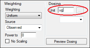
3. In the Weighting/Dosing Options tab below the Setup panel, type ug in the Unit field.
All model estimation procedures benefit from initial estimates of the parameters. While Phoenix can compute initial parameter estimates using curve stripping, this example involves entering values for the initial parameter estimates.
4. Select the Parameter Options tab below the Setup panel.
5. Select the User Supplied Initial Parameter Values option.
The WinNonlin Bounds option is selected by default as the Parameter Boundaries. Do not change this setting.
6. Select Initial Estimates in the Setup panel list.
7. Check the Use Internal Worksheet box.
a. Press OK to accept the default sort variable in the Select sorts dialog.
b. For row 1 (V_F), enter 0.25 in the Initial column.
c. For row 2 (K01), enter 1.81 in the Initial column.
d. For row 3 (K10), enter 0.23 in the Initial column.
Maximum Likelihood Models object
1. Right-click the study1 worksheet in the Data folder and select Send To > Modeling > Maximum Likelihood Models.
2. In the Structure tab, uncheck the Population box.
3. Press the Set WNL Model button.
The contents of the Structure tab changes. The first of the two untitled menus is for selecting a PK model, and the second is for selecting a PD model.
4. In the first untitled menu, select 3 (1cp extravascular).
5. Press Apply to set the WinNonlin model.
6. Map the columns to the contexts as follows:
Subject to Sort.
Time to Time.
Conc to CObs.
The WARNINGS tab at the bottom highlights potential issues. If there are no issues, the tab will be labeled “no warnings”. Click the WARNINGS tab and note the message that Aa values are missing. This will be taken care of in the next few steps.
In this example, a single dose of 2 micrograms was administered at time zero. However, since the concentration units were ng/mL, the dose should be entered as 2000ng so the units are equivalent.
1. Select the Dosing panel in the Setup tab.
2. Check the Use Internal Worksheet box.
a. In the cell under Aa type 2000.
b. In the cell under Time type 0.
3. Press View Source above the worksheet.
4. In the Columns tab below the table:
a. Select Aa from the Columns list.
b. Enter ng in the Unit field.
5. Click X in the upper right corner to close the source window (the units are added to the column header).
Notice that the warning about Aa values is gone and the tab label now says “no warnings.”
The Maximum Likelihood Models engine will not generate its own initial estimates, like the Least-Squares Regression Model engine can, so it is important to consider reasonable starting values.
1. Select the Initial Estimates tab in the lower panel.
2. Extend the Duration to 15, since the last observed timepoint is 14 hours.
3. Enter values 2, 300, and 0.1 for tvKa, tvV, and tvKe, respectively.
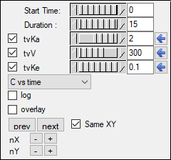
Note: Make sure the tvKe box is checked after entering the value. Entering a leading “0” for a value causes the corresponding checkbox to automatically be cleared.
The y axis can also be set to log scale and, if there is more than one profile, the curves can be overlaid by checking the log and overlay boxes, respectively.
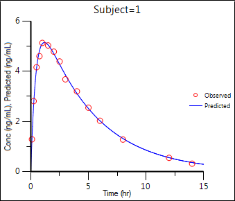
Note how the predicted curve roughly follows the observed data now.

4. Click the blue arrows to submit these values to the main model engine (if the arrow is blue, then the value will not be used).
Execute and view the results
At this point, all of the necessary commands and options have been specified.
1. Execute each object in the workflow.
The Results tab contains three types of model output:
Worksheets (descriptions are located in the “Worksheet output” section)
Plots
Text output
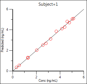
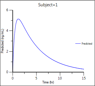
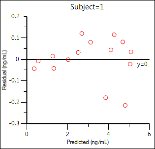
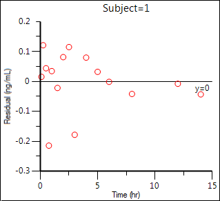
The six plots generated by the PK Model object are shown below. The NLME object generates more plots, however the ones corresponding to the WinNonlin output are listed in parentheses.
Observed Y and Predicted Y vs X (Ind DV, IPRED vs TAD):
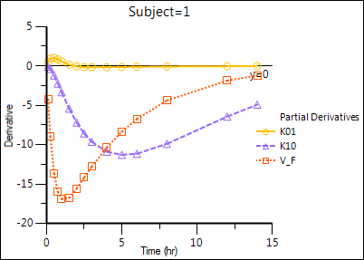
Partial Derivatives plot (Ind Partial Derivatives):
Predicted Y vs Observed Y (Ind DV vs IPRED, axes swapped):
Predicted Y vs X:
Residual Y vs Predicted Y (Ind IWRES vs IPRED):
Residual Y vs X (Ind IWRES vs TAD):
The tables generated by the ML Model object summarize useful information.
Overall: Contains -2LL (the objective function) and other goodness of fit information
Theta: Final parameter estimates
Residuals: Analogous to Summary Table of Least-Squares Regression and NCA models
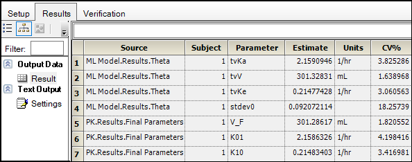
To compare the two models, create a worksheet by appending the Final Parameters worksheet from the PK model to the Theta worksheet from the ML Model object. (See “Append Worksheets” in the worksheet objects documentation for specifics on how to append worksheets.)
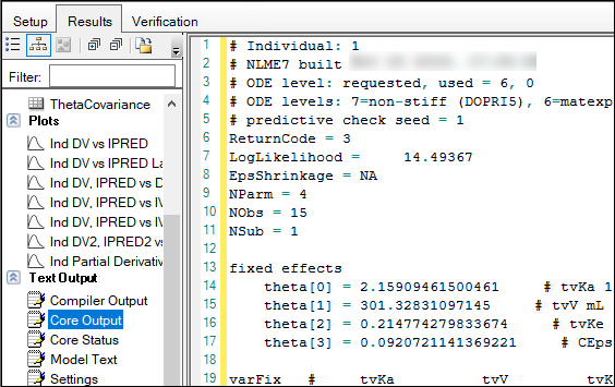
The Core Output text file contains all model settings and output in plain text format. Below is part of the Core Output file from the ML Model object run.
Save the project and the results
Projects and their results can be saved as a project file or loaded into Integral.
To save the project as a file, select File > Save Project.
For details on adding the project to Certara Integral, see ”Adding a savepoint project” on the Integral Assistance website.