CI GEO X% Lower: Lower limit of an X% confidence interval for the logs of the data, back-transformed to original scale:
exp(Mean_Log – ta/2 x SD_Log)
CI GEO X% Upper: Upper limit of an X% confidence interval for the logs of the data, back-transformed to original scale:
exp(Mean_Log + ta/2 x SD_Log)
where (1 – a)*100 is the percentage given for the confidence interval
and ta/2 is from the t-distribution with N – 1 degrees of freedom.
CI X% Lower: Lower limit of an X% confidence interval for the data (i.e., confidence interval that tells the range that is expected to have X% of the data).
Mean – (ta/2 x SD)
CI X% Lower GEO Mean: Lower limit of an X% confidence interval for the Geometric Mean:

(equivalently, exp of the lower CI for Mean_Log).
CI X% Lower Mean: Lower limit of an X% confidence interval for the mean (i.e., the confidence interval in which the mean exists with X% certainty).
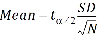
CI X% Lower Var: Lower limit of an X% confidence interval for the variance (i.e., the confidence interval in which the variance exists with X% certainty):
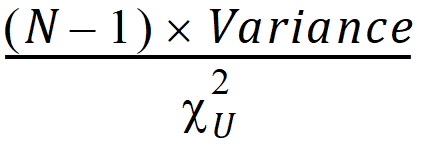
where cu2 is from the c2-distribution with N – 1 degrees of freedom.
cu2 cuts off an upper tail of area a/2 where (1 – a)*100 is the percentage for the confidence interval.
CI X% Upper: Upper limit of an X% confidence interval for the data:

where (1 – a)*100 is the percentage given for the confidence interval
and ta/2 is from the t-distribution with N – 1 degrees of freedom.
CI X% Upper GEO Mean: Upper limit of an X% confidence interval for the Geometric Mean:

where (1 – a)*100 is the percentage given for the confidence interval,
and ta/2 is from the t-distribution with N – 1 degrees of freedom.
CI X% Upper Mean: Upper limit of an X% confidence interval for the mean:
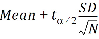
where (1 – a)*100 is the percentage given for the confidence interval
and ta/2 is from the t-distribution with N – 1 degrees of freedom.
Thus, a 95% confidence level indicates that a = 0.05. Note that for N>30, the t-distribution is close to the normal distribution.
CI X% Upper Var: Upper limit of an X% confidence interval for the variance:
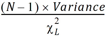
where cL2is from the c2-distribution with N – 1 degrees of freedom.
cL2 cuts off a lower tail of area a/2 where (1 – a)*100 is the percentage for the confidence interval.
CV%: Coefficient of variation:
(SD/Mean)*100
GEO Lower XSD and GEO Upper XSD: Range determined by adding or subtracting “X” log standard deviations from the log-mean, back-transformed to original scale:

When X = 1, this range is equivalent to:
Geometric_Mean/exp(SD_Log) and Geometric_Mean*exp(SD_Log)
Geometric CV%: Geometric coefficient of variation:

Geometric Mean: Nth root of the product of the N observations. Equivalently, the exponential of the Mean_Log. Each value must be > zero:

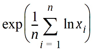
Geometric SD: Geometric standard deviation of the natural logs of the observations exp (SD_Log)
Harmonic Mean: Reciprocal of the arithmetic mean of the reciprocals of the observations:
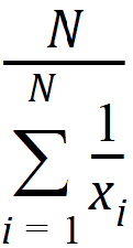
IQR: Interquartile range is the difference between the first and third quartiles (i.e., the middle 50% of the data). IQR is only included in the output when the Include Percentiles box is checked.
KS PValue: Kolmogorov-Smirnov normality test r value. This quantifies the distance between the empirical distribution function of the data and the cumulative distribution function of the Normal distribution. The empirical distribution function Fn for n independent and identically distributed observations Xi is defined as:
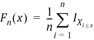
where  is the indicator function and = 1 if
  , otherwise 0.
The Kolmogorov-Smirnov statistic for a given cumulative distribution function F(x) is:

where sup x is the supremum of the set of distances. A r-value is then computed to determine the significance of Dn.
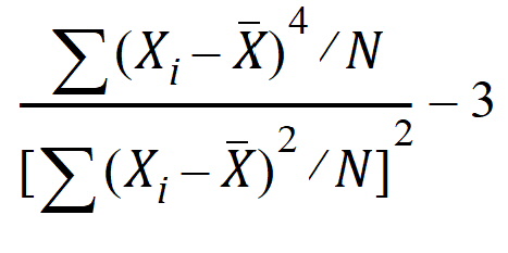
Kurtosis: Sample coefficient of excess (sample excess kurtosis):

Sample Excess Kurtosis = [Population Excess Kurtosis*(N + 1) + 6]*(N – 1)/[(N – 2) x (N – 3)]
Kurtosis Pop: Population coefficient of excess (population excess kurtosis):
Population Excess Kurtosis = ((Sample Excess Kurtosis x (N – 2) x (N – 3)/(N – 1)) – 6)/(N + 1)
Lower XSD and Upper XSD: Range determined by adding or subtracting X standard deviations from the mean Mean +/– X*SD
Max: Maximum value
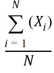
Mean: Arithmetic average
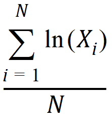
Mean log: Arithmetic average of the natural logs of the observations
Median: Median value — from the percentiles computations, 50th percentile.
Min: Minimum value.
N: Number of observations with non-missing data (i.e., numeric observations).
NMiss: Number of observations with missing data (i.e., non-numeric observations such as text or blanks).
NObs: Number of observations, including observations that are missing or non-numeric (i.e., NObs = N + NMiss)
P(ercentiles): The Pth percentile divides the distribution at a point such that P percent of the distribution are below this point. For a sample size of n, the quantile corresponding to the proportion p (0<p<1) is defined as:
Q(p)=(1 – f)*x(j) + f*x(j + 1)
where:
j = int(p*(n + 1)), (integer part)
f = p*(n + 1) – j, (fractional part)
x(j) = the jth order statistic
The above is used if 1 £ j < n. Otherwise, the empirical quantile is the smallest order statistic for j = 0 or the largest order statistic for j = n.
(Definition 6 in Hyndman and Fan, “Sample Quantiles in Statistical Packages”, American Statistician, Nov 1996. Equivalent to SAS PCTLDEF 4, Excel PERCENTILE.EXC, and NIST Engineering Statistics Handbook, Section 7.2.6.2, Percentiles.)
Pseudo SD: Jackknife estimate of the standard deviation of the harmonic mean. For n points, x1, … xn, the pseudo standard deviation is:
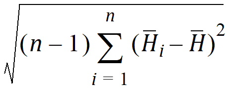
where:
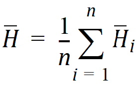
and:
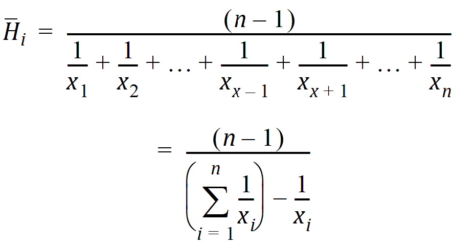
Range: Range of values (maximum value minus minimum value).
SD: Standard Deviation:

SD Log: Standard deviation of the natural logs of the observations:
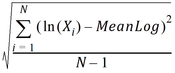
SE: Standard Error:

Skewness: Sample coefficient of skewness (sample skewness):

Sample Skewness=Population Skewness*sqrt(N*(N–1))/(N–2)
Skewness Pop: Population coefficient of skewness (population skewness):
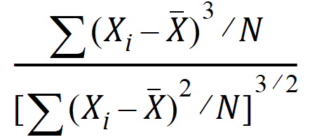
Population Skewness=Sample Skewness*(N–2)/sqrt(N*(N–1))
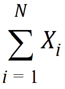
Sum: Sum of the values in the column mapped to Summary:
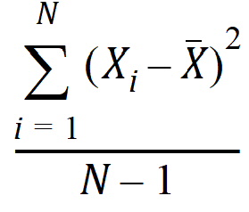
Variance: Unbiased sample variance:
