The methodology is based on linear system analysis with linearity defined in the general sense of the linear superposition principle. It is well recognized that classical linear compartmental kinetic models exhibit superposition linearity due to their origin in linear differential equations. However, all kinetic models defined in terms of linear combinations of linear mathematical operators, such as differentiation, integration, convolution, and deconvolution, constitute linear systems adhering to the superposition principle. The scope and generality of the linear system approach ranges far beyond linear compartmental models.
To fully appreciate the power and generality of the linear system approach, it is best to depart from the typical, physically structured modeling view of pharmacokinetics. To cut through all the complexity and objectively deal with the present problems, it is best to consider the kinetics of drug transport in a non-parametric manner and simply use stochastic transport principles in the analysis.
Convolution/deconvolution — stochastic background
Convolution/deconvolution — stochastic background
The convolution/deconvolution principles applied to evaluate drug release and drug input (absorption) can be explained in terms of point A to point B stochastic transport principles. For example, consider the entry of a single drug molecule at point A at time zero. Let B be a sampling point (a given sampling space or volume) anywhere in the body (e.g. a blood sampling) that can be reached by the drug molecule entering at A. The possible presence of the molecule at B at time t is a random variable due to the stochastic transport principles involved. Imagine repeating this one molecule experiment an infinite number of times and observing the fraction of times that the molecule is at B at time t. That fraction represents the probability that a molecule is at point B given that it entered point A at time zero. Denote this probability by the function g(t).
Next, consider a simultaneous entry of a very large number (N) of drug molecules at time zero, like in a bolus injection. Let it be assumed that there is no significant interaction between the drug molecules, such that the probability of a drug molecule's possible arrival at sampling site B is not significantly affected by any other drug molecule. Then the transport to sampling site B is both random and independent. In addition the probability of being at B at time t is the same and equals g(t) for all molecules. It is this combination of independence and equal probability that leads to the superposition property that in its most simple form reveals itself in terms of dose-proportionality. For example, in the present case the expected number of drug molecules to be found at sampling site B at time t (NB(t)) is equal to Ng(t). It can be seen from this that the concentration of drug at the sampling site B at the arbitrary time t is proportional to the dose. N is proportional to the dose and g(t) does not depend on the dose due to the independence in the transport.
Now further assume that the processes influencing transport from A to B are constant over time. The result is that the probability of being at point B at time t depends on the elapsed time since entry at A but is otherwise independent of the entry time. Thus the probability of being at B for a molecule that enters A at time tA is g(t – tA). This assumed property is called time-invariance. Consider again the simultaneous entry of N molecules but now at time tA instead of zero. Combining this property with those of independent and equal probabilities, i.e., superposition, results in an expected number of molecules at B at time t given by NB(t)=Ng(t – tA).
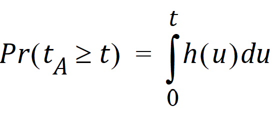
Suppose that the actual time at which the molecule enters point A is unknown. It is instead a random quantity tA distributed according to some probability density function h(t), that is,

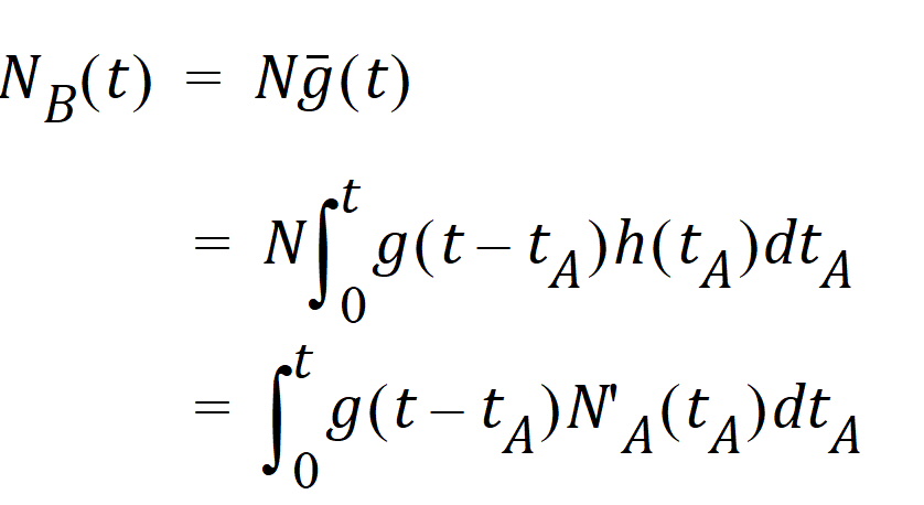
The probability that such a molecule is at point B at time t is the average or expected value of g(t – tA) where the average is taken over the possible values of tA according to:

Causality dictates that g(t) must be zero for any negative times, that is, a molecule cannot get to B before it enters A. For typical applications drug input is restricted to non-negative times so that h(t)=0 for t < 0. As a result the quantity g(t –tA)h(tA) is nonzero only over the range from zero to t and the equation becomes:

Suppose again that N molecules enter at point A but this time they enter at random times distributed according to h(t). This is equivalent to saying that the expected rate of entry at A is given by N’A (t)=Nh(t). As argued before, the expected number of molecules at B at time t is the product of N and the probability of being at B at time t, that is,

Converting from number of molecules to mass units:

where MB(t) is the mass of drug at point B at time t and f(t) is the rate of entry in mass per unit time into point A at time t.
Let Vs denote the volume of the sampling space (point B). Then the concentration, c(t), of drug at B is:

where “*” is used to denote the convolution operation and cd(t) = g(t)/Vs
The above equation is the key convolution equation that forms the basis for the evaluation of the drug input rate, f(t). The function cd(t) is denoted as the unit impulse response, also known as the characteristic response or the disposition function. The process of determining the input function f(t) is called deconvolution because it is required to deconvolve the convolution integral to extract the input function that is embedded in the convolution integral.
The unit impulse response function (cd) provides the exact linkage between drug level response c(t) and the input rate function f(t). cd is simply equal to the probability that a molecule entering point A at t=0 is present in the sampling space at time t divided by the volume of that sample space.
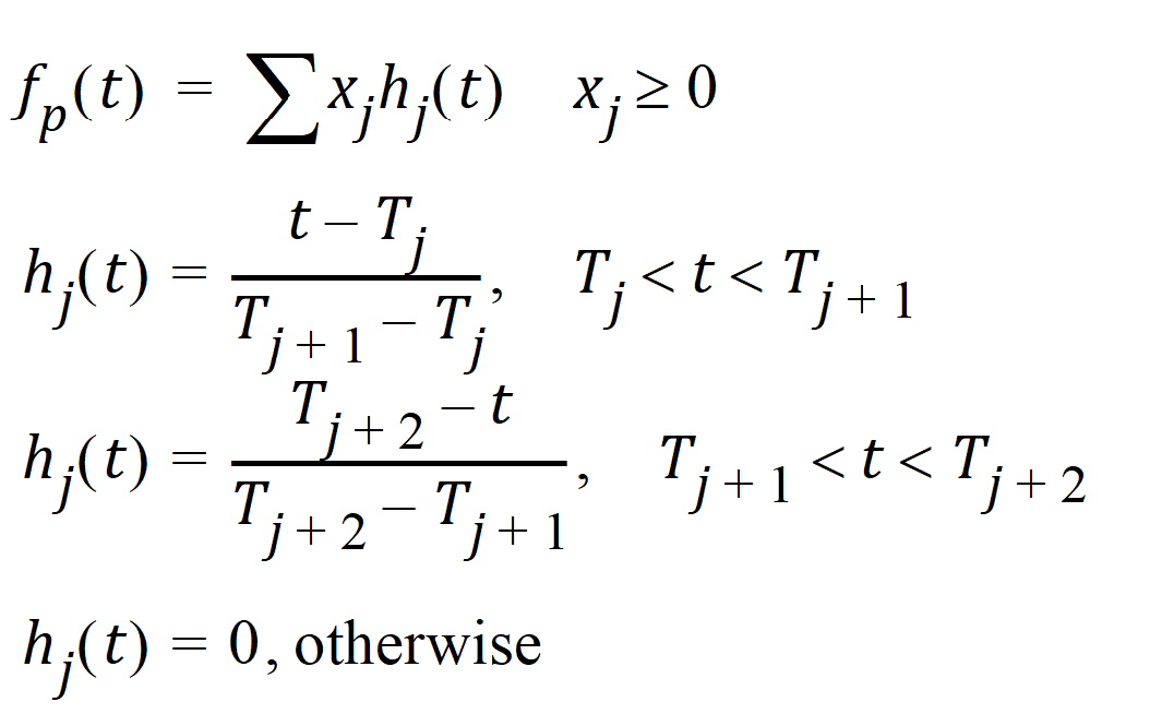
Phoenix models the input function as a piecewise linear “precursor” function fp(t) convolved with an exponential “dispersion” function fd(t). The former provides substantial flexibility whereas the latter provides smoothness. The piecewise linear component is parameterized in terms of a sum of hat-type wavelet basis functions, hj(t):

where xj is the dose scaling factor within a particular observation interval and Tj are the wavelet support points. The hat-type wavelet representation enables discontinuous, finite duration drug releases to be considered together with other factors that result in discontinuous delivery, such as stomach emptying, absorption window, pH changes, etc. The dispersion function provides the smoothing of the input function that is expected from the stochastic transport principles governing the transport of the drug molecules from the site of release to subsequent entry to and mixing in the general systemic circulation.
The wavelet support points (Tj) are constrained to coincide with the observation times, with the exception of the very first support point that is used to define the lag-time, if any, for the input function. Furthermore, one support point is injected halfway between the lag-time and the first observation. This point is simply included to create enough capacity for drug input prior to the first sampling. Having just one support point prior to the first observation would limit this capacity. The extra support point is well suited to accommodate an initial “burst” release commonly encountered for many formulations.
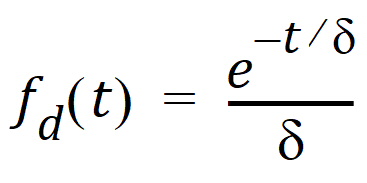
The dispersion function fd(t) is defined as an exponential function:

where d is denoted the dispersion or smoothing parameter. The dispersion function is normalized to have a total integral (t=0 to ¥) equal one, which explains the scaling with the d parameter. The input function, f(t), is the convolution of the precursor function and the dispersion function:

The general convolution form of the input function above is consistent with stochastic as well as deterministic transport principles. The drug level profile, c(t), resulting from the above input function is, according to the linear disposition assumption, given by:

where “*” is used to denote the convolution operation.