Knowledge of how to do basic tasks using the Phoenix interface, such as creating a project and importing data, is assumed.
Fit a PK model to data example
This example is about creating and saving PK models in Phoenix and supposes that a researcher has obtained concentration data from one subject after oral administration of a compound, and now wishes to fit a pharmacokinetic (PK) model to the data.
The completed project (PK_Model.phxproj) is available for reference in …\Examples\WinNonlin.
Explore the PK input data
-
Create a new project.
-
Rename the project as PK Model.
-
Import the file …\Examples\WinNonlin\Supporting files\study1.CSV.
In the File Import Wizard dialog, select the Has units row option and click Finish. -
Right-click Workflow in the Object Browser and select New > Plotting > XY Plot.
-
Drag the study1 worksheet from the Data folder to the XY Data Mappings panel.
Leave Subject mapped to the None context.
Map Time to the X context.
Map Conc to the Y context. -
Click
 to execute the object. The results are displayed on the Results tab.
 -
In the Options tab below the plot, select Axes > Y from the menu tree.
-
Select the Logarithmic option button in the Scale area. Leave the logarithmic base set to 10.
The XY Plot is automatically updated to reflect the scale change.
Set up the object
The plots suggests that the system might be adequately modeled by a one-compartment, 1st order absorption model. This model is available as Model 3 in the pharmacokinetic models included in Phoenix. Set up a PK Model object and a Phoenix Model object, for comparison.
PK Model object
-
Right-click Workflow in the Object Browser and select New > WNL 5 Classic Modeling > PK Model.
-
With the new PK Model object selected in the Object Browser, drag the study1 worksheet from the Data folder to the Main Mappings panel.
Map Subject to the Sort context.
Leave Time mapped to the Time context.
Map Conc to the Concentration context. -
In the Model Selection tab below the Setup panel, check the Number 3 model checkbox.
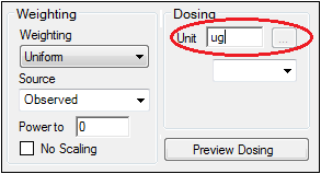
Entering the units for dosing data makes it possible to view and adjust units for the model parameters.
In this example, a single dose of 2 micrograms was administered at time zero.
-
Select the Dosing panel in the Setup tab.
-
Check the Use Internal Worksheet checkbox.
-
Click OK in the Select sorts dialog to accept the default sort variable.
-
In the cell under Time type 0.
-
In the cell under Dose type 2.
-
In the Weighting/Dosing Options tab below the Setup panel, type ug in the Unit field.
All model estimation procedures benefit from initial estimates of the parameters. While Phoenix can compute initial parameter estimates using curve stripping, this example will provide user values for the initial parameter estimates.
-
Select the Parameter Options tab below the Setup panel.
-
Select the User Supplied Initial Parameter Values option.
The WinNonlin Bounds option is selected by default as the Parameter Boundaries. Do not change this setting. -
Select Initial Estimates in the Setup panel list.
-
Check the Use Internal Worksheet checkbox.
-
Click OK to accept the default sort variable in the Select sorts dialog.
-
Enter the following information in the table:
For row 1 (V_F), enter 0.25 in the Initial column.
For row 2 (K01), enter 1.81 in the Initial column.
For row 3 (K10), enter 0.23 in the Initial column.
-
Right-click the study1 worksheet in the Data folder and select Send To > Phoenix Modeling > Phoenix Model.
-
In the Structure tab, uncheck the Population box.
-
Click the Set WNL Model button.
The contents of the Structure tab changes. The first of the two untitled menus allows users to select a PK model, and the second allows users to select a PD model. -
In the first untitled menu, select 3 (1cp extravascular).
-
Click Apply to set the WinNonlin model.
-
Use the option buttons in the Main Mappings panel to map the data types to the following contexts:
Subject to the Sort context.
Time to the Time context.
Conc to the CObs context.
The WARNINGS tab at the bottom highlights potential issues. If there are no issues, the tab will be labeled “no warnings”. Click the WARNINGS tab and note the message that Aa values are missing. This will be taken care of in the next few steps.
In this example, a single dose of 2 micrograms was administered at time zero. However, since the concentration units were ng/mL, the dose should be entered as 2000ng so the units are equivalent.
-
Select the Dosing panel in the Setup tab.
-
Check the Use Internal Worksheet checkbox.
-
In the cell under Aa type 2000.
-
In the cell under Time type 0.
-
Click View Source above the worksheet.
-
In the Columns tab below the table, select Aa from the Columns list and enter ng in the Unit field.
-
Click X in the upper right corner to close the source window (the units are added to the column header).
Notice that the warning about Aa values is gone and the tab label now says “no warnings.”
The NLME engine will not generate its own initial estimates, like the WNL Classic engine can, so it is important to consider reasonable starting values.
-
Select the Initial Estimates tab in the lower panel.
-
Extend the Duration to 15, since the last observed timepoint is 14 hours.
-
Enter values 2, 300, and 0.1 for tvKa, tvV, and tvKe, respectively.
-
Click the blue arrows to submit these values to the main model engine (if the arrow is blue, then the value will not be used).
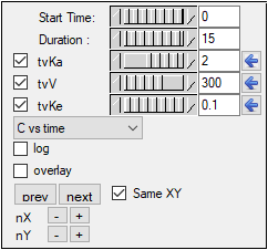
The y axis can also be set to log scale and, if there is more than one profile, the curves can be overlaid by checking the log and overlay boxes, respectively.
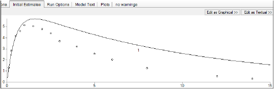
Note how the predicted curve roughly follows the observed data now.
Execute and view the results
At this point, all of the necessary commands and options have been specified.
-
Select the Workflow object in the Object Browser and click
 to execute the all objects in the workflow. The results are displayed in the Results tab.
The Results tab contains three types of model output:
•Worksheets (descriptions of the worksheets are located in the “Worksheet output” section)
•Plots
•Text output
The six plots generated by the PK Model object are shown below. The NLME object generates more plots, however the ones corresponding to the WinNonlin output are listed in parentheses.
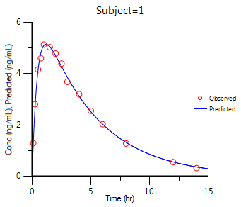
Observed Y and Predicted Y vs X (Ind DV, IPRED vs TAD)
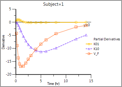
Partial Derivatives plot (Ind Partial Derivatives)
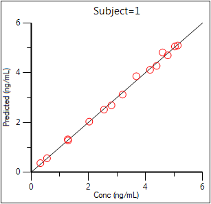
Predicted Y vs Observed Y (Ind DV vs IPRED, axes swapped)
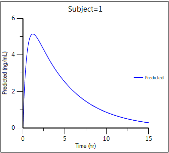
Predicted Y vs X
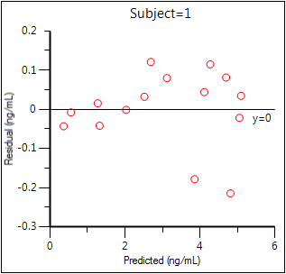
Residual Y vs Predicted Y (Ind IWRES vs IPRED)
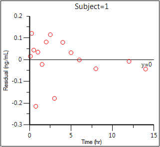
Residual Y vs X (Ind IWRES vs TAD)
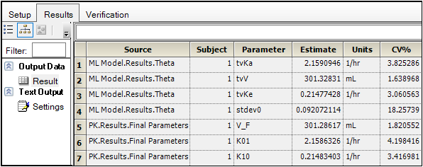
The tables generated by the Phoenix Model summarize useful information.
•Overall: Contains -2LL (the objective function) and other goodness of fit information
•Theta: Final parameter estimates
•Residuals: Analogous to Summary Table of WNL classic and NCA models
To compare the two models, create a worksheet by appending the Final Parameters worksheet from the PK model to the Theta worksheet from the Phoenix Model. (See “Append Worksheet” for specifics on how to append worksheets.)
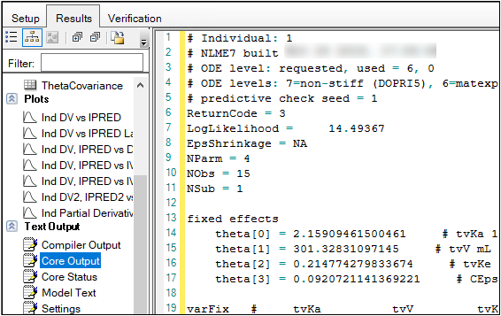
The Core Output text file contains all model settings and output in plain text format. Below is part of the Core Output file from the Phoenix Model run.
Save the project and the results
Projects and their results can be saved as a project file or loaded into Integral.
To save the project as a file:
-
Select File > Save Project.
-
In the Save Project dialog, select a directory in the Save in menu or use the default directory.
-
Type a name in the File name field or use the default name and click Save.
-
Close the project by right-clicking the project in the Object Browser and selecting Close Project.
The project is saved as a Phoenix Project (.phxproj) file.
For details on adding the project to Certara Integral, see “Adding a project to Integral”.
Simulation and study design of PK models example
Considerable research has been done in the area of optimal designs for linear models. Most methods involve computation of the variance covariance matrix. The “optimal” design is usually one in which replicate samples are taken at a limited number of combinations of experimental conditions. Unfortunately, these methods are of little or no value when designing experiments involving nonlinear models for a number of reasons, including:
•It can be difficult or, in the case of a pharmacokinetic study, impossible to obtain replicate observations.
•The primary interest often is not in the model parameters but in some functions of the model parameters such as AUC, t1/2, etc.
When Phoenix performs a simulation, the output includes information on precisely how parameters in the model can be estimated for specified values of the independent variables, such as time.
Assume that a study is being planned and that the data produced by this study should be consistent with Phoenix PK model 3. Assume also that the parameter values should be approximately: V_F=10, K01=3, K10=0.05 and one of the following study designs, or sampling times, will be used:
0, 1.5, 3, 6, 9, 12, 15, 18, and 24 hours
or
0, 0.5, 1, 2, 4, 8, 12, 24, and 36 hours.
Simulation can be used to determine which set of sampling times would produce the more precise estimates of the model parameters. This example will use Phoenix to simulate the model with each set of sampling times, and compare the variance inflation factors for the two simulations.
The completed project (Study_Design.phxproj) is available for reference in …\Examples\WinNonlin.
Create the input dataset
-
Create a new project with the name Study Design.
-
Right-click the Data folder in the Object Browser and select New > Worksheet.
-
Name the new worksheet Example Data.
-
In the Columns tab, add a column identifying the group number by clicking Add underneath the Columns list.
-
In the New Column Properties dialog, type Group in the Column Name field. Leave the data type set to Numeric, and click OK.
-
In the first cell under Group, type 1 and press ENTER. Continue to enter 1 for rows 2–9.
-
In rows 10–18 type 2 in the Group column.
-
Add a column of time data by clicking Add underneath the Columns list.
-
In the Column Name field, type Times. Leave the data type set to Numeric and click OK.
-
Type the values 0, 1.5, 3, 6, 9, 12, 15, 18, and 24 in the Times column for rows 1–9 and values 0, 0.5, 1, 2, 4, 8, 12, 24, and 36 for rows 10–18. (Alternatively, the data can be imported from …\Examples\WinNonlin\Supporting files\Example Data.csv.
This model is available as Model 3 in the pharmacokinetic models included in Phoenix.
-
Right-click Workflow and select New > WNL5 Classic Modeling > PK Model.
-
Drag the Example Data worksheet from the Data folder to the Main Mappings panel.
Map Group to the Sort context.
Map Times to the Time context. -
In the Model Selection tab below the Setup panel, specify the PK model that Phoenix will use in the analysis by selecting the Number 3 model checkbox.
-
Select the Simulation checkbox on the right side of the Model Selection tab (notice that the Concentration mapping is changed from required (orange) to option (gray)).
-
In the Y Units field, type ng/mL.
-
Enter the dosing data by selecting the PK Model's Dosing panel in the Setup tab.
-
Check the Use Internal Worksheet checkbox.
-
Click OK in the Select sorts dialog to accept the default sort variable.
-
In the Time column type 0 for both groups.
-
In the Dose column type 100 for both groups.
-
In the Weighting/Dosing Options tab below the Setup panel, type mg in the Unit field.
-
Select the Parameter Options tab.
Parameter values must be specified for simulations. The User Supplied Initial Parameter Values option is selected and cannot be changed. The Do Not Use Bounds option is selected by default and cannot be changed.
Selecting the Simulation checkbox makes the parameter calculation and boundary selection options unavailable. If the Simulation checkbox is selected, then users must supply initial parameter values, and parameter boundaries are not used. -
Select Initial Estimates in the Setup list.
-
Check the Use Internal Worksheet checkbox.
-
In the Select sorts dialog, click OK to accept the default sort variable.
-
Enter the following initial values for each group: V_F=10, K01=3, K10=0.05.
Note:The number of rows in the Group column corresponds to the number of doses received. For example, if group 1 had 10 doses, there would be 10 rows of dosing information for group 1. In Phoenix this grouping of data is referred to as stacking data.
Execute and view the results
All the settings are complete and the model can be executed.
-
Click
 to execute the object.
The variance inflation factors (VIF) for each dosing scheme (groups 1 and 2) are located in the Final Parameters worksheet and are summarized (with values rounded) in the following table.
|
Parameter |
Estimate |
Group 1 VIF |
Group 2 VIF |
|
V_F |
10 |
0.779 |
0.657 |
|
K01 |
3 |
68.48 |
1.176 |
|
K10 |
0.05 |
0 |
0 |
In practice, it is useful to vary the values of V_F, K01, and K10 and repeat the simulations to determine if the first set of sampling times consistently yields less precise estimates than the second set.
Design the sampling plan
Note that, for the parameters V_F and K10, the estimated variances would be approximately 15% lower using the second set of times, while the difference is much more dramatic for the parameter K01. These sets of variance inflation factors indicate that the second set of sampling times would provide tighter estimates of the model parameters.
The partial derivatives plots for this model explain this result. The locations at which the partial derivative plots reach a maximum or a minimum indicate times the model is most sensitive to changes in the model parameters, so one approach to designing experiments is to sample where the model is most sensitive to changes in the model parameters.
-
Click Partial Derivatives Plot in the Results tab.
-
Select the Page 02 tab below the plot.
-
Close this project by right-clicking the project and selecting Close Project.
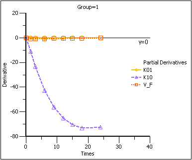
Partial Derivatives plot Group 1
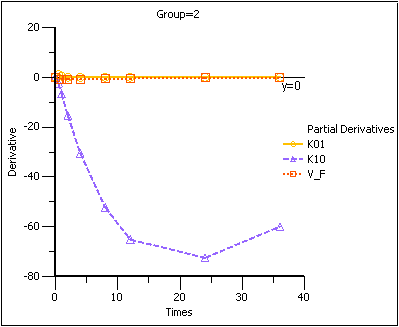
Note that in the first plot of the partial derivatives the model is most sensitive to changes in K10 at about 20 hours. Both sampling schemes included times near 20 hours, so therefore the two sets of sampling times were nearly equivalent in the precision with which K10 would be estimated.
For both V_F and K01 the model is most sensitive to changes very early, at about 0.35 hours for K01 and about 1.4 hours for V_F. The first set of sampling times does not include any post-zero points until hour 3, long past these areas of sensitivity. Even the second set of times could be improved if samples could be taken earlier than 0.5 hours.
This same technique could be used for other models in Phoenix or for user-defined models.
More WNL5 Classic modeling examples
Knowledge of how to do basic tasks using the Phoenix interface, such as creating a project and importing data, is assumed.
The examples project Model_Examples.phxproj located in …\Examples\WinNonlin involve WNL5 classic modeling objects. Each model object within this project contains the appropriate default mappings and settings needed to run the model.
To run these example objects:
-
Load the project …\Examples\WinNonlin\Model_Examples.phxproj into Phoenix.
Each example model has the following items associated with it: -
Explore each model object and its mappings and settings.
-
Click
 to execute each model. The results are displayed on the Results tab.
•A dataset in workbook form.
•Many have datasets in workbook form for dosing.
•A PK, PKPD, Indirect Response, or an ASCII model object.
Explanations for each model object in the example is given below.
Pharmacokinetic model (Exp1)
In the Exp1 example, a dataset was fit to PK model 13 in the pharmacokinetic model library. Four constants are required for model 13: the stripping dose associated with the parameter estimates, the number of doses, the dose, and the time of dosing.
This example uses weighted least squares (1/observed Y). Phoenix determines initial estimates via curve stripping and then generates bounds for the parameters.
Pharmacokinetic model with multiple doses (Exp2)
In the Exp2 example, a dataset obtained following multiple dosing is fit to model 13 in the pharmacokinetic model library, which is a two-compartment open model. This model has five parameters: A, B, K01, Alpha, and Beta and uses the user-supplied initial values 20, 5, 3, 2, and 0.05. Phoenix generates bounds for the parameters.
Probit analysis: maximum likelihood estimation of potency (Exp3)
The Exp3 example demonstrates how to use the NORMIT and WTNORM functions to perform a probit regression (parallel line bioassay or quantal bioassay) analysis. Note that a probit is a normit plus five. There are several interesting features used in this example:
-
The transform capability was used to create the response variable.
-
The logarithm of the relative potency is estimated as a secondary parameter.
-
Maximum likelihood estimates were obtained by iteratively reweighting and turning off the halvings and convergence criteria. Therefore, instead of iterating until the residual sum of squares is minimized, the program adjusts the parameters until the partial derivatives with respect to the parameters in the model are zero. This will normally occur after a few iterations.
-
Since there is no s2 in a problem such as this, variances for the maximum likelihood estimates are obtained by setting S2=1 (MEANSQUARE=1).
-
The following modeling options are used:
•Method 3 is selected, which is recommended for Maximum Likelihood estimation (MLE), and iterative reweighting problems.
•Convergence Criterion is set to 0. This turns off convergence checks for MLE.
•Iterations are set to 10. Estimates should converge after a few iterations.
•Meansquare is set to 1. Sigma squared is 1 for MLE.
For further reading regarding use of nonlinear least squares to obtain maximum likelihood estimates, refer to Jennrich and Moore (1975). Maximum likelihood estimation by means of nonlinear least squares. Amer Stat Assoc Proceedings Statistical Computing Section 57–65.
Logit regression (bioassay) (Exp4)
The following data were obtained in a toxicological experiment:
|
Dose (mg) |
# DoseD (n) |
# Died (Y) |
|
300 |
50 |
15 (30%) |
|
1000 |
20 |
9 (45%) |
|
3300 |
26 |
19 (73%) |
|
10000 |
12 |
12 (100%) |
In the Exp4 example, assume that the distribution of Y is binomial with:
mean=np
variance=npq, and q=1 – p
where 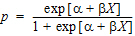 and X=loge dose
Maximum likelihood estimates of a and b for this model are obtained via iteratively reweighted least squares. This is done by fitting the mean function (np) to the Y data with weight (npq) –1.
The modeling commands needed to fit this model to the data are included in an ASCII model file. Note that the loge LD50 and loge LD001 are also estimated as secondary parameters.
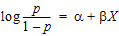
This model is really a linear logit model in that:
|
|
(1) |
Note:For this type of problem, the final value of the residual sum of squares is the Chi-square statistic for testing heterogeneity of the model. If this example is run a user obtains X2 (heterogeneity)=2.02957, with 4 – 2=2 degrees of freedom (number of data points minus the number of parameters that were estimated).
For a more in-depth discussion of the use of nonlinear least squares for maximum likelihood estimation, see Jennrich and Moore (1975). Maximum likelihood estimation by means of nonlinear least squares. Amer Stat Assoc Proceedings Statistical Computing Section 57–65.
In the Engine Settings tab, the Convergence Criteria is set to zero to turn off the halving and convergence checks. Meansquare is set to 1 (the residual mean square is redefined to be 1.00) in order to estimate the standard errors of a, b, and the secondary parameters.
Survival analysis (Exp5)
Exp5 is another maximum likelihood example and is very similar to Model Exp4. It is included to show that models arising in a variety of disciplines, such as case survival or reliability analysis, can be fit by nonlinear least squares.
The dosing constant is defined in this model as the denominator for the proportions, that is, N.
In the Engine Settings tab the Convergence Criteria is set to zero to turn off the halving and convergence checks. Meansquare is set to 1 (redefines the residual mean square to be 1.00) in order to estimate the standard errors of the primary and secondary parameters.
Two differential equations with data for both compartments (Exp6)
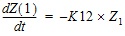
Exp6 involves the following model:
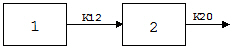
where K12 and K20 are first-order rate constants. This model may be described by the following system of two differential equations.
|
|
(2) |
 compartment 1
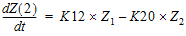 compartment 2
with initial conditions Z1=D, and Z2=0.
In addition to obtaining estimates of K12 and K20, it is also desirable to estimate D and the half-lives of K12 and K20.
A sample solution for this example is given here. Note that, for this example, the model is defined as an ASCII file. Data corresponding to both compartments are available.
Column C in the dataset for this example contains a function variable, which defines the separate functions.
Two differential equations with data on one-compartment (Ex7)
The model for the Exp7 example is identical to that for Exp6. However, in this example, it is assumed that data are available only for compartment two.
Multiple linear regression (Exp8)
Linear regression models are a subset of nonlinear regression models; consequently, linear models can also be fit using Phoenix. To illustrate this, a sample dataset (taken from Analyzing Experimental Data By Regression by Allen and Cady (1982), Lifetime Learning Publications, Belmont, CA) was analyzed in Exp8. Note that linear models can always be written as:
|
|
(3) |
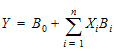
This example is also interesting in that the model was initially defined in such a way to permit several different models to be fit to the data.
In the ASCII model panel, note that the number of parameters to be estimated is defined in CONS in order to make the model specification as general as possible. Note also the use of a DO loop in the model text.
Note:When using Phoenix to fit a linear regression model:
- use arbitrary initial values
- make sure the Do Not Use Bounds option is checked
- select the Gauss-Newton minimization method with the Levenberg and Hartley modification
The dosing constant for this example is the number of terms to be fit in the regression.
Cumulative areas under the curve (Exp9)
The Exp9 example uses the TRANSFORM block of commands to output cumulative area under the curve values calculated by trapezoidal rule. It computes cumulative urine excretion then fits it to a one-compartment model. The use of the LAG function is demonstrated.
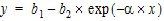
Mitscherlich nonlinear model (Exp10)
In the Exp10 example, a dataset is fit to the Mitscherlich model. The data were taken from Allen and Cady (1982), Analyzing Experimental Data By Regression. Lifetime Learning Publications, Belmont, CA. Fitting data to this model involves the estimation of three parameters; b1, b2, and a.
|
|
(4) |
Four parameter logistic model (Exp11)
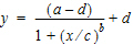
The Exp11 example illustrates how to fit a dataset to a general four parameter logistic function. The function is often used to fit radioimmunoassay data. The function, when graphed, depicts a sigmoidal (S-shaped) curve. The four parameters represent the lower and upper asymptotes, the ED50, and a measure of the steepness of the slope. For further details see DeLean, Munson and Rodbard (1978). Simultaneous analysis of families of sigmoidal curves: Application to bioassay, radioligand assay and physiological dose-response curves. Am J Physiol 235(2):E97–E102. The model, with parameters a, b, c, and d is as follows:
|
|
(5) |
Linear regression (Exp12)
The Exp12 example is based on work published by Draper and Smith (1981). Applied Regression Analysis, 2nd ed. John Wiley & Sons, NY.
Note:When doing linear regression in Phoenix, enter arbitrary initial estimates and make sure the Do Not Use Bounds option is checked. Use the Gauss-Newton minimization method with the Levenberg and Hartley modification
Indirect response model (IR)
The IR example is PD8 from the textbook: Gabrielsson and Weiner (2016). Pharmacokinetic and Pharmacodynamic Data Analysis: Concepts and Applications, 5th ed. Apotekarsocieteten, Stockholm. It uses an indirect response model, linking Phoenix pharmacokinetic model 11 to indirect response model 54. The PK data were fit in a separate run and are linked to the Indirect Response model. This can be done via the PKVAL command when using an ASCII model or via the PK parameters panel. Model 11 is a two-compartment micro constant model with extravascular input.
Ke0 link model (PKPD)
The PKPD example is PD10 from the textbook: Gabrielsson and Weiner (2016). Pharmacokinetic and Pharmacodynamic Data Analysis: Concepts and Applications, 5th ed. Apotekarsocieteten, Stockholm. It uses an effect compartment PK/PD link model. The drug was administered intravenously, and a one-compartment model is assumed (PK Model 1). The PD data is fit to a simple Emax model (PD Model 101). The pharmacokinetic data were fit in a separate run and are linked to the pharmacodynamic model.
Pharmacokinetic/pharmacodynamic link model (Exp15)
Rather than fitting the PK data to a PK model, an effect compartment is fitted and Ke0 estimated in the Exp15 example using the observed Cp data. Therefore it is a type of nonparametric model. The collapsed Ce values are then used to model the PD data. The example also illustrates how to mix differential equations and integrated functions. This approach was proposed by Dr. Wayne Colburn.
