Example - Model using logarithmic concentration values

Model using logarithmic concentration values (Lyon dataset)

The data used in the Lyon dataset is from a simulated trial. The concentration data is the logarithm of the concentration data. In this model the logarithm of each prediction value is used to predict the concentration values.

Note:The completed project (Lyon05.phxproj) is available for reference in …\Examples\NLME.

Set up the Phoenix model object

Create a new project called Lyon05.
Import the dataset …\Examples\NLME\Supporting files\lyon05dose.dat.
Click Finish in the File Import Wizard dialog.
Right-click the lyon05dose worksheet and select Send To > Modeling > Maximum Likelihood Models.
In the Structure tab, select Micro from the Parameterization menu.
In the Absorption menu, select Extravascular.

Map the model variables

Select the option buttons in the Main Mappings panel to map the data types as follows:
xid to the ID context.
time to the Time context.
dose to the Aa context.
yobs to the Cobs context.

Edit the graphical model

Click Edit as Graphical.
In the confirmation dialog, click Yes.
In a second confirmation dialog about not using the closed-form, click Yes.
If needed, click Model in the Setup tab list to display the Model diagram panel.

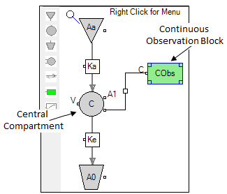
Delete the connector between the Continuous Observation block CObs and the Central compartment C.
Left-click the square in the middle of the connector to select it.
Right-click the square and select Delete.
Confirm the deletion by clicking Yes in the dialog.
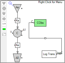
Add a Procedure block by right-clicking anywhere in the Model diagram panel and select Insert > Procedure.
A Procedure block named Proc1 is added to the Model diagram.
In the Name field in the Structure tab, type Log Trans.
In the Code sub-tab of the Structure tab, type logC=log(C) in the Code field.
Left-click the Log Trans output square, labeled logC, and drag it to the input square of the Continuous Observation block, labeled C.

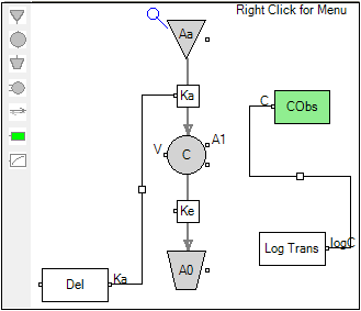
Right-click anywhere in the Model diagram panel and select Insert > Procedure to add a second Procedure block.
In the Name field, type Del.
In the Code sub-tab, type Ka=Ke+Del in the Code field.
Select the Str. Parameters sub-tab and click Add.
In the field, type Del.
In the Model diagram panel, left-click the Del output square, labeled Ka, and drag it to the input square of Ka PK flow, labeled Ka.

Note:Connecting Del’s Ka output to PK flow Ka’s input changes Ka from a structural parameter to an output parameter.

Select the Parameters > Secondary sub-tab.
Click Add.
Type tvKa in the Parameter field.
Type tvKe+tvDel in the Definition field.
Select the Random Effects sub-tab.
Clear the Diag checkbox to use a full block structure.
Select the Fixed Effects sub-tab.
Enter the following initial estimates:
tvV = 25
tvKe = 0.3
tvDel = 0.3
Select the Run Options tab.
Select FOCE L-B as the algorithm.
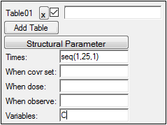
Select Add Table. The table definition fields are displayed.
In the Times field, type seq(1,25,1).
In the Variables field, type C.

Click (Execute icon) to execute the object.

Run the model using a different engine

Although the FOCE L-B model engine was used, the Lyon data is also valid for use with the QRPEM model engine. As a continuation of this example, create a copy of the Maximum Likelihood Models object and use the QRPEM method to generate results.

Right-click the ML Model object in the Object Browser and select Copy.
Right-click on the Workflow object in the Object Browser and select Paste.
Rename the Copy of ML Model object to QRPEM Model.

All of the mappings and other settings are retained in the QRPEM Model object, so the only change needed is to select QRPEM as the engine.
Click the Run Options tab.
Select QRPEM from the Algorithm menu.
Execute the object.

Save and close the project

Select File > Save Project.
Click Save.
Select File > Close Project.

The project is saved and closed and Phoenix can be safely exited.

This concludes the modeling with logarithmic concentration values example.