An example of individual modeling with Maximum Likelihood Model object
This example illustrates how a dataset can be fitted to a two-compartment model with first-order absorption in the pharmacokinetic model library using either the Least-Squares Regression PK Model or a Maximum Likelihood Models object GUI.
Exp1 data is used, which is a dataset fit to PK model 13 in the pharmacokinetic model library. Four constants are required for model 13: the stripping dose associated with the parameter estimates, the number of doses, the dose, and the time of dosing.
Note:The completed project (IndivPK.phxproj) is available for reference in …\Examples\NLME.
Set up the Least-Squares Regression PK model object
-
Create a new project called IndivPK.
-
Import the datasets IndivPK11.xls and IndivPK11_Dose.xls from …\Examples\NLME\Supporting files.
-
In the File Import Wizard dialog, click the Next Arrow button to move from the IndivPK11 dataset to IndivPK11 and click Finish.
-
Right-click the IndivPK11 worksheet and select Send To > Modeling > Least Squares Regression Models > PK Model.
-
Rename the object as WNL Model.
-
Use the option buttons in the Main Mappings panel to map the data types to the following contexts:
Time to the Time context.
Conc to the Concentration context. -
Click Dosing in the Setup tab.
-
Use the mouse pointer to drag the IndivPK11_Dose worksheet from the Data folder to the Main Mappings panel. Data types should automatically map as follows:
Time to the Time context.
Dose to the Dose context. -
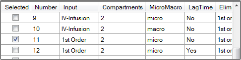
In the Model Selection tab, scroll down the table of models and check the box for model 11.
-
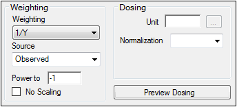
Select the Weighting/Dosing Options tab.
-
In Weighting menu select 1/Y.
-
Click
 (Execute icon) to execute the object.
Create the Maximum Likelihood model object
-
Right-click the IndivPK11 worksheet and select Send To > Modeling > Maximum Likelihood Models.
-
Rename the object as NLME Model.
-
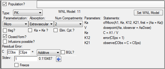
In the Structure tab, uncheck the Population box.
-
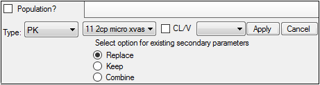
Click the Set WNL Model button.
The contents of the Structure tab changes. The first of the two untitled menus allows users to select a PK model, and the second allows users to select a PD model. -
In the first untitled menu, select Model 11 (11 2cp micro xvas).
-
Make sure the second untitled menu is clear and click Apply to set the model.
-
Use the option buttons in the Main Mappings panel to map the data types to the following contexts:
Time to the Time context.
Conc to the CObs context. -
Click Dosing in the Setup tab.
-
Use the mouse pointer to drag the IndivPK11_Dose worksheet from the Data folder to the Main Mappings panel.
-
Use the option buttons in the Dosing Mappings panel to map the data types to the following contexts:
Dose to the Aa context.
Time to the Time context. -
Execute the object.
Initial Estimates configuration
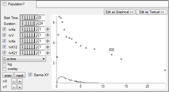
The Initial Estimates tab can be used to find the best initial estimates for different parameters.
-
Select the Initial Estimates tab.
Adjust the portion of the plot to view using the Start Time and Duration options. -
For this example, set the Duration to 24 either using the slider or typing the value in the field next to the slider.
-
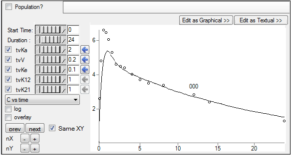
Enter different values for the fixed effect parameters, as shown in the table below, and see how each adjustment affects the results on the XY plot. Use the slider or typing the value in the field next to the slider.
tvKa = 2
tvV = 0.2 (make sure to re-check the checkbox)
tvKe = 0.1 (make sure to re-check the checkbox)
tvK12 = 1
tvK21 = 1 -
Click the left arrow button beside each parameter to copy the new estimate to the Initial estimate field.
For more information on using the Initial Estimates, see the “Initial Estimates tab” description. -
Execute the object.
Comparing the results
-
Open the Theta worksheet in the Results tab for the Phoenix Model object.
-
Open Final Parameters worksheet in the Results tab of the WNL Model object.
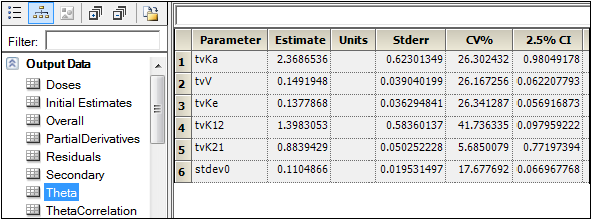
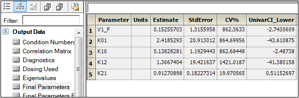
The names of parameters in Maximum Likelihood Models have the following equivalents in the PK Model.
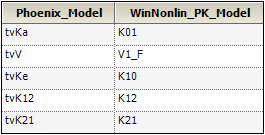
Compare the results of estimated fixed effects. As one can see, the estimates in these models are close but not equal due to different method of model fitting.
This concludes the individual modeling example.
