Using a linked indirect response model
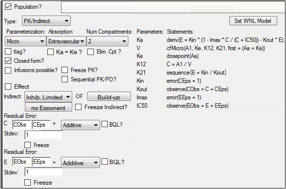
The data in link-IPR.dat consists of measured effect values over time in 10 subjects, following a single dose at time zero. Effect is measured at the same 14 time points in all subjects. A reasonable fit is obtained utilizing a two-compartment model with first-order absorption linked to an indirect response model with inhibition of input, both of which are available as Least-Squares Regression PK model 11 and Indirect Response model 51.
The effect is modeled as a function of the drug concentration in the central compartment, Cp, and parameters representing the measured response to the drug, R, a zero-order constant for production of response, Kin, a first-order rate constant for loss of response, Kout, and the drug concentration at half-maximum inhibition, IC50.
Within-subject error is assumed independently distributed with constant variance.
Note:The completed project (Linked_IPR.phxproj) is available for reference in …\Examples\NLME.
Set up the Maximum Likelihood Models object
-
Name the new project Linked IPR.
-
Import the dataset …\Examples\NLME\Supporting files\link-IPR.dat.
Click Finish in the File Import Wizard dialog. -
Right-click the worksheet and select Send To > Modeling > Maximum Likelihood Models.
-
In the Structure tab of the Maximum Likelihood Models object, select PK/Indirect from the Type menu.
-
Select Micro from the Parameterization menu.
-
In the Absorption menu, select Extravascular.
-
In the Num Compartments menu, select 2.
-
In the Indirect menu, select Inhib. Limited.
-
Select the Parameters > Structural sub-tab.
-
Clear the Ran checkbox beside Imax to remove any random effects from the parameter.
-
Select the Fixed Effects sub-tab.
-
Enter the following initial estimates:
tvKa = 0.92
tvV = 2.44
tvKe = 0.44
tvK12 = 0.36
tvK21 = 0.24
tvKin = 400
tvKout = 2
tvImax = 1
tvIC50 = 15 -
Check the Freeze checkbox beside tvImax to freeze the parameter.
-
Select the Run Options tab.
-
In the Algorithm menu, select Naive pooled.

Map the model variables and dosing
-
Use the option buttons in the Main Mappings panel to map the data types to the following contexts:
time to the Time context.
subject to the ID context.
effect to the EObs context. -
Click Dosing in the Setup tab.
-
In the Dosing Mappings panel, turn on the Use Internal Worksheet checkbox.
-
In the table, enter 100 in the first cell of the Aa column.
-
Enter 0 in the first cell of the Time column.
-
Select the two cells containing the values just entered and drag the selection to the include all rows.
When the mouse button is released, all rows in the table will have “100” and “0” values for the Aa and Time columns, respectively. -
Click
 (Execute icon) to execute the object.
 -
In the Results tab, check the Core Output text file. The fixed effect value for epsilon (EEps) is used as the standard deviation for the epsilon error model in the next model execution.
Change the model to full block
-
Select the Structure tab.
-
Click
 beside the E Stdev field to use the new value for residual error.
 -
Select the Parameters > Random Effects sub-tab.
-
Clear the Diag checkbox to create a full block model.
-
Select the Run Options tab.
-
In the Algorithm menu, select FOCE L-B.
-
Execute the object.
This concludes the linked indirect response modeling example.
