The Phoenix Model Object

Phoenix Model computations

Differential equations in NLME
Sequential PK/PD Population Model Fitting
Prediction and Prediction Variance Corrections
Shrinkage calculation

Differential equations in NLME

Ordinary differential equations can be solved by Phoenix models by several methods. These methods can be selected under the option Max ODE in the Input Options tab.

Matrix Exponent option
Stiff/Non-Stiff options — LSODE (Livermore Solver)
Auto-Detect option — LSODA
RTOL, ATOL, and MAXSTEP ODE error controls

Matrix Exponent option

This is the default option for solving ordinary equations for Phoenix models. The general N-compartment model governed by ordinary differential equations takes the form:

(1)

where y(t) =(y1(t), …, yN(t))T is an N-dimensional column vector of amounts in each compartment as a function of time, f(y) is a column vector-valued function which gives the structural dependence of the time derivatives of y on the compartment amounts, and r is an n-dimensional column vector of infusion rates into the compartments. Note that as opposed to the closed-form solution first-order models, dosing can be made into any combination of compartments, and all of the compartments are modeled.

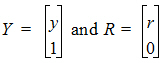
To account for infusion rates, define the augmented system Y=[y, 1], and R=[r, 0]. In the special first-order case, the equations are represented as Y=JY where J is the Jacobian matrix:

(2)

The partial derivatives are obtained by symbolic differentiation of f(Y). If any of them are not constant (over the given time interval), matrix exponent cannot be used, and an ODE solver is used.

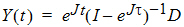
The state vector Y evolves according to:

(3)

where e^Jt is defined by the Taylor series expansion of the standard exponential function. Standard math library routines are available for the computation of the matrix exponential. These are faster and more accurate than the equivalent computation with a numerical ODE solver and do not suffer from stiffness.

In the steady state case where a vector bolus dose is given at intervals of length, the solution takes the form:

(4)

where D is a column vector giving the amount of the bolus deposited in each compartment.

If matrix exponent cannot be used, the steady state is found by pre-running the model via the ODE solver for enough multiples of t so that Y changes by less than a tolerance.

Stiff/Non-Stiff options — LSODE (Livermore Solver)

LSODE (Livermore Solver for Ordinary Differential Equations) is the basic ODE solver for the Phoenix model. It solves stiff and non-stiff systems of the form dy/dt=f. In the stiff case, it treats the Jacobian matrix df/dy as either a dense (full) or a banded matrix, and as either user-supplied or internally approximated by difference quotients. It uses Adams methods (predictor-corrector) in the non-stiff case, and Backward Differentiation Formula (BDF) methods (the Gear methods) in the stiff case. The linear systems that arise are solved by direct methods (LU factor/solve).

Stiff systems typically arise from models with processes that proceed at very different rates, for example, very slow equilibration of a peripheral compartment with a central compartment relative to the rate at which elimination occurs from the central compartment. Generally, a stiff solver outperforms, in terms of both time and accuracy, a non-stiff solver for such systems, but the non-stiff solver can be superior for non-stiff systems.

Phoenix also solves ODE systems, when possible, by the matrix exponential method. This method requires that the system be expressible as dy/dt=Jy, where J is a matrix (the Jacobian) with elements that are constant over a time interval. This is the default solver. If the J matrix cannot be derived from the differential equations, the system automatically reverts to the non-stiff solver.

In the Run Options tab in the Phoenix model, there are four different methods for obtaining ODE solutions, three of which use the LSODE methodology:

LSODE nonstiff solver (Fastest)
LSODE stiff solver with a Jacobian internally approximated by difference quotients, if expressions are not differentiable. LSODE stiff solver with an explicitly supplied Jacobian, if expressions are differentiable and constant. The Phoenix model supplies the Jacobian in this form if it can.
Matrix exponential, which is the default option.

If a requested level does not apply, for example if matrix exponential is requested but the model is not linear, then Phoenix attempts to use the next lower level that is applicable.

Note:If a nonstiff solver is used (equivalent to ADVAN6 in NONMEM), level 1 must be specified.

Auto-Detect option — LSODA

Nonlinear systems can change from still to non-stiff during evaluation which can result in incorrect estimates and/or much longer execution times if the incorrect ODE solver is selected. The auto-detect option is an ordinary differential equation integrator (LSODA written by Linda R. Petzold and Alan C. Hindmarsh) that automatically detects if the nonlinear system is stiff or non-stiff and chooses the appropriate method. LSODA is a very robust adaptive stepwise solver that uses the nonstiff method initially, and dynamically monitors data in order to decide which method to use.

RTOL, ATOL, and MAXSTEP ODE error controls

The ODE (ordinary differential equation) numerical solvers used by Phoenix have three accuracy controls that are available to the user in the “Advanced” Run Options tab:

Ode Rel. Tol.: Relative tolerance (RTOL)
RTOL=|<computed value> – <true solution value>|/|<computed value>|
Ode Abs. Tol.: Absolute tolerance (ATOL)
ATOL=|<computed value> – <true solution value>|
Ode max step: Maximum number of internal allowable steps (MAXSTEP) to achieve the above accuracies.

The default values for ATOL and RTOL are 0.000001, while the default value of MAXSTEP is 50000.

If RTOL is set to 0.0, then only ATOL is applied by the ODE solver (pure absolute error control). Similarly, in the case of the non-stiff solver, if ATOL is set to 0.0, only RTOL is applied by the solvers (pure relative error control). Currently, the use of pure relative error control for the stiff and auto-detect solvers is not permitted and can lead to errors. Note both tolerances are local controls on the current integration interval, and the global error may exceed these values. For a more complete discussion of error controls in ODE solvers, see Hindmarsh, Alan C., “ODEPACK, A Systematized Collection of ODE Solvers,” Scientific Computing, R. S. Stepleman et al (eds.), North-Holland, Amsterdam (1983) pp. 55–64.

For Matrix Exponential, which only applies to the special, but very important and common case in PK/PD models of linear differential equations with constant rate coefficients, only an absolute tolerance ATOL applies. If ATOL is set to zero, it is reset internally to the square root of the machine precision (approximately 1.e–8). For a full discussion, see Sidje, Roger B., “EXPOKIT – A Matrix Package for Computing Matrix Exponentials,” ACM Transactions on Mathematical Software, 24 (1998) pp. 130–156.

Sequential PK/PD Population Model Fitting

Sequential PK/PD fitting in a built-in model
Sequential PK/PD fitting in a graphical model
Sequential PK/PD fitting in a textual model

Sequential PK/PD fitting in a built-in model

Generally, fitting a PK/PD model with population data is best done with a combined model, where the input data contains both PK observations (plasma concentration) and PD observations (effect). However, if it is desired to fit the model sequentially, for reasons of performance or modeling stability, that can also be done. This is done by creating two models, one for the PK model alone, and one for PK/PD, where the PK part of the second model imports data from the results of the first model.

Create the PK-only model and fit it against the combined input data set, ignoring the effect observations.

•The Sort Input? option in the Run Options tab must be checked.

•Refine the model until it is considered satisfactory.

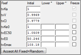
•Be sure to select Accept All Fixed + Random under the Parameters > Fixed Effects tab, so that the estimated values are transferred to the initial values.

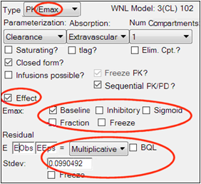
Copy the PK-only model to a second model and convert it to a PK/Emax model under the Structure tab.

This ensures that the PK portion of the second model is identical to the PK-only model. It must be identical in structure, have the same structural, fixed effect, and random effect parameters, and initial estimates. It must also have the identical main input datasets, mapped in the identical way.
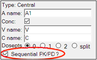
Check the Sequential PK/PD? option on the Structure tab.

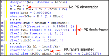
Checking the Sequential PK/PD option has the effect of freezing the PK portion of the model, and turning its random effects into covariates to be imported from the first model, so that plasma concentration will be predicted identically to what it was predicted as in the first model. It also removes the PK observation from the model, since the PK portion of the model is not being fit.

Note:Frozen fixed effects are not allowed to have random effects in the model text generated from built-in or graphical models. This may cause confusion because the user interface may appear as if random effects on fixed effects are supported. See “User interface settings and the sequential PK/PD” for more information.

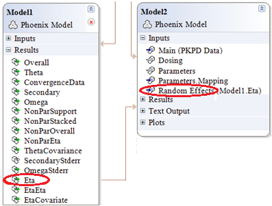
Map the Eta output of the first model to the Random Effects input of the second model.

Make sure the mapping is completed correctly:

•Scenario is mapped to None.

•ID is mapped to ID.

•nV is mapped to nV.

•nCl is mapped to nCl.

Set up the PD portion of the model.

Look at the Fixed Effects tab. When the model is run, it will only fit the fixed and random effects for the PD portion of the model. The PK parameters are not estimated because they come from the first model:

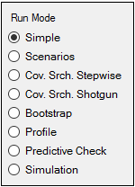
Look at the Run Options tab. All run modes can be used. Note that Scenarios and the two Cov. Srch. modes will only apply to covariate effects in the PD portion of the model. PK covariate effects must be unchanged from the first model. In the Profile mode, the only fixed effects available for profiling are the PD fixed effects.

User interface settings and the sequential PK/PD

The user interface settings may appear to allow random effects on fixed effects, even though this situation is not supported. For example, if random effects for PK parameters are selected first, then the corresponding fixed effects are frozen, the user interface will appear as if random effects on fixed effects are allowed, since both checkboxes are selected, but the model text will not have these random effects.

In addition, the interface allows Sequential PK/PD? to be selected without having any random effects in the model. In this case, the model will execute without error, even though it is not a true sequential PK/PD model, since random effects from the PK model are not being used. The Ran checkboxes for the corresponding fixed effects need to be selected prior to selecting the Sequential PK/PD? checkbox in order to run as a true sequential PK/PD model.

If a user wants to run a sequential PK/PD model and, due to loading an existing project or due to freezing fixed effects prior to checking Sequential PK/PD?, the interface is in a state where Sequential PK/PD is selected, and the Freeze PK? checkbox or the Freeze checkboxes for the fixed effects are selected and disabled (thereby removing the random effects from the model text), the user must:

1. Unselect Sequential PK/PD

2. Unselect the Freeze PK? checkbox or the Freeze checkboxes for the fixed effects

3. Select the Ran checkboxes for the corresponding fixed effects (if not already selected)

4. Re-select Sequential PK/PD?

5. Map the random effects on the Random Effects mappings panel on the Setup tab

Sequential PK/PD fitting in a graphical model

To convert the second model to graphical, it is recommended to first set it up in built-in mode, and then use Edit as Graphical.

The resulting graphical model has no PK observation:

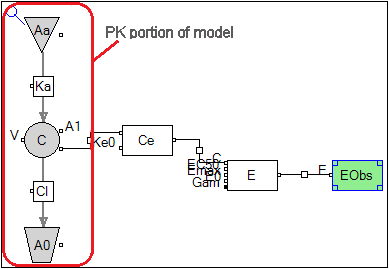
Every component of the PK model has a checkbox called Sequential PK/PD which is checked.

This checkbox causes the parameters associated with that compartment or flow to be treated as frozen, with imported random effects. (This is necessary because a graphical model is more modifiable than a built-in model. Since the user may make changes, they must tell NLME which components are PK components.) When the graphical model is generated from the built-in model, these options are automatically set.

The PD portion of the model can be modified as desired. The remaining usage is the same as that described for the built-in model.

Sequential PK/PD fitting in a textual model

To make a textual model equivalent to a built-in or graphical model, it is recommended to start with a built-in or graphical set up and then select Edit as Textual.

The text shows the result:

Now the PD portion may be modified as desired, and executed as in the built-in or graphical models.

Prediction and Prediction Variance Corrections

Including a prediction correction and prediction variance correction as part of predictive checking allows observations that would otherwise be incomparable to be pooled together to narrow the quantiles of predicted data, making a more stringent test for possible model misspecification. For example, by using time-after-dose (TAD) as the X axis, data following multiple dose events can be combined. If doses are given at widely varying dose amounts, predictions of plasma concentrations will be proportionally scaled together (assuming a linear model). Similarly, variability correction may apply if, for example, the model is linear but the error model is additive.

Prediction and prediction variance corrections deal with these quantities:

•Y_ij: j^th observation for i^th subject

•PRED_ij: Population (zero-eta) prediction of j^th observation for i^th subject

•PRED_bin: Median of PRED_ij over all observations in a particular bin

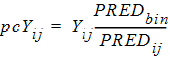
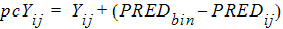
•pcY_ij: Prediction-corrected version of j^th observation for i^th subject

The prediction-corrected observation is calculated either by the proportional rule (default):

(5)

or by the additive rule:

(6)

Further, if Pred. Variance is selected, these variables come into play:

•sd(pcY_ij): Standard deviation of pcY_ij

•sd(pcY_bin): Median of sd(pcY_ij) over the bin

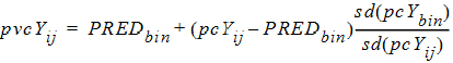
•pvcY_ij: Prediction-variability corrected version of Y_ij

pvcY_ij is calculated as follows:

(7)

Then either the quantity pvcY_ij or pcY_ij is used in the predictive-check plots, depending on whether Pred. Variance is selected.

Shrinkage calculation

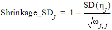
The Omega output worksheet contains h shrinkage data. It is based on the standard deviation definition:

(8)

where SD(h_j) is the empirical standard deviation of the j^th h over all Nsub subjects, and w_j,j is the estimate of the population variance of the j^th random effect, j = 1,2,..., NEta.

For all population engines other than QRPEM, the numerical h_j value used in the shrinkage computation is the mode (maximum) of the empirical Bayesian posterior distribution of the random effects h_j, evaluated at the final parameter estimates of the fixed and random effects. For QRPEM, the h_j value is the mean of the empirical Bayesian distribution.

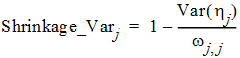
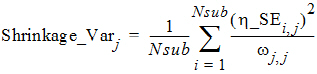
It is worth pointing out that another common way to define the h-shrinkage is through the variance, and is given by

(9)

where Var(h_j) is the empirical variance of the j^th h over all Nsub subjects. By Eqs. (8) and (9), one can see that standard deviation based h-shrinkage can be computed from variance based h-shrinkage, and vice versa. For example, if one has Shrinkage_Var_j, then Shrinkage_SD_j can be calculated as:

(10)

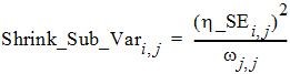
The Eta output worksheet contains the individual shrinkage, which is calculated as follows:

(11)

where i = 1, 2, ..., Nsub and j = 1, 2, ..., NEta. Here, h_SE_i,j denotes the standard error of the j^th individual parameter estimator for the i^th subject. For all population engines other than QRPEM, h_SE_i,j is calculated as the square root of the (j, j)^th element of the inverse of the negative Hessian (second derivative matrix) of the empirical Bayesian posterior distribution for the i^th subject. While, for the QRPEM engine, they are computed via the importance sampling of the empirical Bayesian posterior distribution.

The formula used to calculate Shrink_Sub_Var (11) is extended from the 1-1 relation between the population shrinkage and standard error of individual parameter estimator conjectured in Xu, et al, AAPS J., (2012) pp. 927-936. This relationship can be intuitively observed from the following important theoretical relationship obtained for the EM algorithm.

(12)

From which, one can see that the commonly used variance based population shrinkage, (9), becomes

(13)

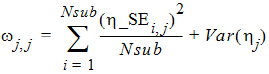
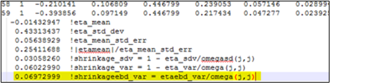
It is worth pointing out that population shrinkage calculated using the above formula, (13), is also reported in bluptable.dat (after the individual shrinkages for each h), and is denoted as shrinkageebd_var (see the highlighted text in yellow in the image below). From these results, we can see that the value of shrinkageebd_var is similar to the one for Shrinkage_Var.

In bluptable.dat, Shrink_Sub_SD is calculated by using the following formula

(14)

This relationship between Shrink_Sub_SD and Shrink_Sub_Var is an analog of the relationship shown in (10).