The general N-compartment model governed by ordinary differential equations takes the form:

where y(t) =(y1(t), …, yN(t))T is an N-dimensional column vector of amounts in each compartment as a function of time, f(y) is a column vector-valued function which gives the structural dependence of the time derivatives of y on the compartment amounts, and r is an n-dimensional column vector of infusion rates into the compartments. Note that as opposed to the closed form solution first-order models, dosing can be made into any combination of compartments, and all of the compartments are modeled.
To account for infusion rates, define the augmented system Y=[y, 1], and R=[r, 0]. In the special first-order case, the equations are represented as:

where J is the Jacobian matrix:
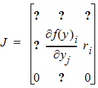
The partial derivatives are obtained by symbolic differentiation of f(Y). If any of them are not constant over the given time interval, then matrix exponent cannot be used, and a numerical ODE solver is used. The case where J is constant requires that the overall differential equation system is linear with no explicit time dependencies, that is, the system can be described by a series of fixed inter-compartmental rate constants which are the entries in the matrix J.
Note that any model (such as Michaelis-Menten) with at least one nonlinear flow does not satisfy the constant J condition and must be solved with a numerical ODE solver.
Assuming J is a constant, the state vector Y evolves according to:
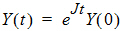
where eJt is defined by the Taylor series expansion I+Jt+(Jt)2/2! +… of the standard exponential function. Standard math library routines are available for the computation of the matrix exponential. These are faster and more accurate than the equivalent computation with a numerical ODE solver and do not suffer from stiffness.
For steady state computations, regardless of whether a matrix exponential or numerical ODE solution is used for the single dose case, repeated dosing cycles are made to allow the system to approach steady state within a specified tolerance. An extrapolation technique known as Aitken acceleration is used to accelerate the convergence of steady state computations so that usually only a few such cycles are needed to achieve high accuracy steady state results.
