Therapeutic response

For non-compartmental analysis of concentration data, Phoenix computes additional parameters for different time range computations, as listed below. The parameters included depend on whether upper, lower, or both limits are supplied. See “Therapeutic response windows” for additional computa­tion details.

Time range from dose time to last observation 
Additional parameters:

TimeLow: Total time below lower limit. Included when lower or both limits are specified.
TimeBetween: Total time between lower/upper limits. Included when both limits are specified.
TimeHigh: Total time above upper limit. Included when lower or both limits are specified.
AUCLow: AUC that falls below lower limit: Included when lower or both limits are specified.
AUCBetween: AUC that falls between lower/upper limits. Included when both limits are specified.
AUCHigh: AUC that falls above upper limit. Included when lower or both limits are specified.

Time range from dose time to infinity using Lambda Z (if Lambda Z exists)
Additional parameters:

TimeInfBetween: Total time (extrapolated to infinity) between lower/upper limits. Included when both limits are specified.
TimeInfHigh: Total time (extrapolated to infinity) above upper limit. Included when lower or both limits are specified.
AUCInfLow: AUC (extrapolated to infinity) that falls below lower limit: Included when lower or both limits are specified.
AUCInfBetween: AUC (extrapolated to infinity) that falls between lower/upper limits. Included when both limits are specified.
AUCInfHigh: AUC (extrapolated to infinity) that falls above upper limit. Included when lower or both limits are specified.

Therapeutic response windows 

For therapeutic windows, one or two boundaries for concentration values can be given, and the pro­gram computes the time spent in each window determined by the boundaries and computes the area under the curve contained in each window. To compute these values, for each pair of consecutive data points, including the inserted point at dosing time if there is one, it is determined if a boundary crossing occurred in that interval. Call the pair of time values from the dataset (t_i, t_i+1) and called the boundaries y_lower and y_upper.

If no boundary crossing occurred, the difference t_i+1, t_i is added to the appropriate parameter TimeLow, TimeBetween, or TimeHigh, depending on which window the concentration values are in. The AUC for (t_i, t_i+1) is computed following the user’s specified AUC calculation method as described in the section on the “Options tab”. Call this AUC*. The parts of this AUC* are added to the appropriate parameters AUCLow, AUCBetween, or AUCHigh. For example, if the concentra­tion values for this interval occur above the upper boundary, the rectangle that is under the lower boundary is added to AUCLow, the rectangle that is between the two boundaries is added to AUC­Between and the piece that is left is added to AUCHigh. This is equivalent to these formulae:

AUCLow = AUCLow + y_lower(t_i+1 – t_i)

AUCBetween = AUCBetween + (y_upper – y_lower)(t_i+1 – t_i)

AUCHigh = AUCHigh + AUC* – y_upper(t_i+1 – t_i)

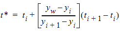
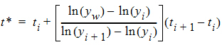
If there was one boundary crossing, an interpolation is done to get the time value where the cross­ing occurred; call this t*. The interpolation is done by either the linear rule or the log rule following the user’s AUC calculation method as described in the section on the “Options tab”, i.e., the same rule is used as when inserting a point for partial areas. To interpolate to get time t* in the interval (t_i, t_i+1) at which the concentration value is y_w:

Linear interpolation rule for time:

 

Log interpolation rule for time:

 

The AUC for (t_i, t*) is computed following the user’s specified AUC calculation method. The differ­ence t* – t_i is added to the appropriate time parameter and the parts of the AUC are added to the appropriate AUC parameters. Then the process is repeated for the interval (t*, t_i+1).

If there were two boundary crossings, an interpolation is done to get t* as above for the first boundary crossing, and the time and parts of AUC are added in for the interval (t_i, t*) as above. Then another interpolation is done from t_i to t_i+1 to get the time of the second crossing t** between (t*, t_i+1), and the time and parts of AUC are added in for the interval (t*, t**). Then the times and parts of AUC are added in for the interval (t**, t_i+1).

The extrapolated times and areas after the last data point are now considered for the therapeutic win­dow parameters that are extrapolated to infinity. For any of the AUC calculation methods, the AUC rule after tlast is the log rule, unless an endpoint for the interval is negative or zero in which case the linear rule must be used. The extrapolation rule for finding the time t* at which the extrapolated curve would cross the boundary concentration y_w is:

 

If the last concentration value in the dataset is zero, the zero value was used in the above compu­tation for the last interval, but now ylast is replaced with the following if Lambda Z is estimable:

y_last = exp(Lambda_z_intercept – Lambda_z(t_last))

If ylast is in the lower window: InfBetween and InfHigh values are the same as Between and High values. If Lambda Z is not estimable, AUCInfLow is missing. Otherwise:

AUCInfLow = AUCLow + (y_last / Lambda_z)

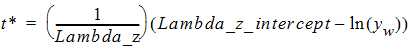
If ylast is in the middle window for two boundaries: InfHigh values are the same as High values. If Lambda Z is not estimable, InfLow and InfBetween parameters are missing. Otherwise: Use the extrapolation rule to get t* at the lower boundary concentration. Add time from tlast to t* into TimeInfBetween. Compute AUC* from tlast to t*, add the rectangle that is under the lower bound­ary into AUCInfLow, and add the piece that is left into AUCInfBetween. Add the extrapolated area in the lower window into AUCInfLow. This is equivalent to:

t* = (1/Lambda_z)(Lambda_z_intercept – ln(y_lower))

TimeInfBetween = TimeBetween + (t* – t_last)

AUCInfBetween = AUCBetween + AUC* – y_lower(t* – t_last)

AUCInfLow = AUCLow + y_lower(t* – t_last) + y_lower / Lambda_z

If ylast is in the top window when only one boundary is given, the above procedure is followed and the InfBetween parameters become the InfHigh parameters.

If there are two boundaries and y_last is in the top window: If Lambda Z is not estimable, all extrap­olated parameters are missing. Otherwise, use the extrapolation rule to get t* at the upper boundary concentration value. Add time from tlast to t* into TimeInfHigh. Compute AUC* for tlast to t*, add the rectangle that is under the lower boundary into AUCInfLow, add the rectangle that is in the mid­dle window into AUCInfBetween, and add the piece that is left into AUCInfHigh. Use the extrapola­tion rule to get t** at the lower boundary concentration value. Add time from t* to t** into TimeInfBetween. Compute AUC** from t* to t**, add the rectangle that is under the lower bound­ary into AUCInfLow, and add the piece that is left into AUCInfBetween. Add the extrapolated area in the lower window into AUCInfLow. This is equivalent to:

t* = (1/Lambda_z)(Lambda_z_intercept – ln(y_upper))

t** = (1/Lambda_z)(Lambda_z_intercept – ln(y_lower))

TimeInfHigh = TimeHigh + (t* – t_last)

TimeInfBetween = TimeBetween + (t** – t*)

AUCInfHigh = AUCHigh + AUC* – y_upper(t* – t_last)

AUCInfBetween = AUCBetween
     + AUC* + (y_upper – y_lower)(t* – t_last)
     + AUC** – y_lower(t** – t*)

AUCInfLow = AUCLow + y_lower(t* – t_last)
     + y_lower(t** – t*) + y_lower / Lambda_z

---

Last modified date:7/9/20

Legal Notice | Contact Certara
© 2020 Certara USA, Inc. All rights reserved.