Simulation and study design of PK models example

Considerable research has been done in the area of optimal designs for linear models. Most methods involve computation of the variance covariance matrix. The “optimal” design is usually one in which replicate samples are taken at a limited number of combinations of experimental conditions. Unfortunately, these methods are of little or no value when designing experiments involving nonlinear models for a number of reasons, including:

•It can be difficult or, in the case of a pharmacokinetic study, impossible to obtain replicate observations.

•The primary interest often is not in the model parameters but in some functions of the model parameters such as AUC, t_1/2, etc.

When Phoenix performs a simulation, the output includes information on precisely how parameters in the model can be estimated for specified values of the independent variables, such as time.

Assume that a study is being planned and that the data produced by this study should be consistent with Phoenix PK model 3. Assume also that the parameter values should be approximately: V_F=10, K01=3, K10=0.05 and one of the following study designs, or sampling times, will be used:

0, 1.5, 3, 6, 9, 12, 15, 18, and 24 hours
or
0, 0.5, 1, 2, 4, 8, 12, 24, and 36 hours.

Simulation can be used to determine which set of sampling times would produce the more precise estimates of the model parameters. This example will use Phoenix to simulate the model with each set of sampling times, and compare the variance inflation factors for the two simulations.

The completed project (Study_Design.phxproj) is available for reference in …\Examples\WinNonlin.

Create the input dataset

Follow the following steps to create the dataset. Alternatively, the data can be imported from …\Examples\WinNonlin\Supporting files\Example Data.csv.

Create a new project with the name Study Design.
Right-click the Data folder in the Object Browser and select New > Worksheet.
Name the new worksheet Example Data.
In the Columns tab, add a column identifying the group number by clicking Add underneath the Columns list.
In the New Column Properties dialog, type Group in the Column Name field. Leave the data type set to Numeric, and click OK.
In the first cell under Group, type 1 and press ENTER. Continue to enter 1 for rows 2–9.
In rows 10–18 type 2 in the Group column.
Add a column of time data by clicking Add underneath the Columns list.
In the Column Name field, type Times. Leave the data type set to Numeric and click OK.
Type the values 0, 1.5, 3, 6, 9, 12, 15, 18, and 24 in the Times column for rows 1–9 and values 0, 0.5, 1, 2, 4, 8, 12, 24, and 36 for rows 10–18.

Set up the object

This model is available as Model 3 in the pharmacokinetic models included in Phoenix.

Right-click Example Data in the Data folder and select Send To > Modeling > Least Squares Regression Models > PK Model.
In the Main Mappings panel:
Map Group to the Sort context.
Map Times to the Time context.
In the Model Selection tab below the Setup panel, specify the PK model that Phoenix will use in the analysis by selecting the Number 3 model checkbox.
Select the Simulation checkbox on the right side of the Model Selection tab (notice that the Concentration mapping is changed from required (orange) to option (gray)).
In the Y Units field, type ng/mL.
Enter the dosing data by selecting the PK Model's Dosing panel in the Setup tab.
Check the Use Internal Worksheet checkbox.
Click OK in the Select sorts dialog to accept the default sort variable.
In the Time column type 0 for both groups.
In the Dose column type 100 for both groups.

Note:The number of rows in the Group column corresponds to the number of doses received. For example, if group 1 had 10 doses, there would be 10 rows of dosing information for group 1. In Phoenix this grouping of data is referred to as stacking data.

In the Weighting/Dosing Options tab below the Setup panel, type mg in the Unit field.
Select the Parameter Options tab.

Parameter values must be specified for simulations. The User Supplied Initial Parameter Values option is selected and cannot be changed. The Do Not Use Bounds option is selected by default and cannot be changed.

Selecting the Simulation checkbox makes the parameter calculation and boundary selection options unavailable. If the Simulation checkbox is selected, then users must supply initial parameter values, and parameter boundaries are not used.
Select Initial Estimates in the Setup list.
Check the Use Internal Worksheet checkbox.
In the Select sorts dialog, click OK to accept the default sort variable.
Enter the following initial values for each group: V_F=10, K01=3, K10=0.05.

Execute and view the results

All the settings are complete and the model can be executed.

Execute the object.

The variance inflation factors (VIF) for each dosing scheme (groups 1 and 2) are located in the Final Parameters worksheet and are summarized (with values rounded) below.

V_F
    Estimate = 10
    Group 1 VIF = 0.779
    Group 2 VIF = 0.657

K01
    Estimate = 3
    Group 1 VIF = 68.48
    Group 2 VIF = 1.176

K10
    Estimate = 0.05
    Group 1 VIF = 0
    Group 2 VIF = 0

In practice, it is useful to vary the values of V_F, K01, and K10 and repeat the simulations to determine if the first set of sampling times consistently yields less precise estimates than the second set.

Design the sampling plan

Note that, for the parameters V_F and K10, the estimated variances would be approximately 15% lower using the second set of times, while the difference is much more dramatic for the parameter K01. These sets of variance inflation factors indicate that the second set of sampling times would provide tighter estimates of the model parameters.

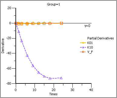
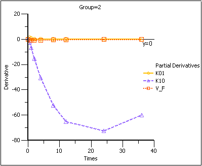
The partial derivatives plots for this model explain this result. The locations at which the partial derivative plots reach a maximum or a minimum indicate times the model is most sensitive to changes in the model parameters, so one approach to designing experiments is to sample where the model is most sensitive to changes in the model parameters.

Click Partial Derivatives Plot in the Results tab.

Partial Derivatives plot Group 1

Select the Page 02 tab below the plot.

Note that in the first plot of the partial derivatives the model is most sensitive to changes in K10 at about 20 hours. Both sampling schemes included times near 20 hours, so therefore the two sets of sampling times were nearly equivalent in the precision with which K10 would be estimated.

For both V_F and K01 the model is most sensitive to changes very early, at about 0.35 hours for K01 and about 1.4 hours for V_F. The first set of sampling times does not include any post-zero points until hour 3, long past these areas of sensitivity. Even the second set of times could be improved if samples could be taken earlier than 0.5 hours.

This same technique could be used for other models in Phoenix or for user-defined models.

Close this project by right-clicking the project and selecting Close Project.