Semicompartmental model example

This example uses the dataset in the file PK.CSV, which is located in the Phoenix examples directory. The data are from an early Phase I PK/PD trial. Quick input is sought for the design of a seven day multiple dose study. However, the profiles are irregular, and it is not easy to apply a compartmental modeling approach to the data. A semicompartmental approach will be attempted here. This example then continues with a NonParametric Superposition prediction of plasma concentrations and effect-site concentrations at steady-state, using the Semicompartmental results (see “NonParametric Superposition example”.

Knowledge of how to do basic tasks using the Phoenix interface, such as creating a project and importing data, is assumed.

The completed project (SCM.phxproj) is available for reference in …\Examples\WinNonlin.

Explore the input data

Create a new project called SCM.
Import the file …\Examples\WinNonlin\Supporting files\PK.CSV.
In the File Import Wizard dialog, select the Has units row option.

The braces in the Effect column header indicate that the units are nonstandard and will be carried throughout the analysis but they cannot be used in unit conversions.
Right-click PK in the Data folder and select Send To > Plotting > XY Plot.
In the XY Data Mappings panel:
Map Subject to the Group context.
Map Time to the X context.
Map Conc to the Y context.
Leave Effect mapped to None.
Click (Execute icon) to execute the object.

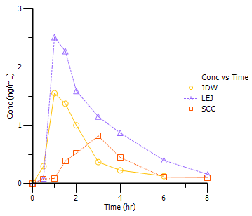
The plot indicates that compartmental modeling might be problematic. The data are highly variable.

Return to the Setup panel and re-map the input data:
Leave Subject mapped to the Group context.
Map Time to None.
Map Conc to the X context.
Map Effect to the Y context.
In the Options tab below the Setup panel, select Graphs > Effect vs Conc in the menu tree.
Clear the Sort X Values checkbox.

Clearing the Sort X Values checkbox tells Phoenix to not sort the dataset by ascending concentration values before creating the XY plot.
Execute the object.

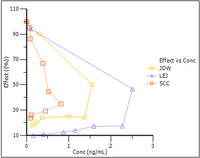
Notice the hysteresis in the plot. Semicompartmental modeling supports calculation of effect-site concentrations based on Ke0. In this example, pre-clinical studies indicated that the Ke0 is between 0.2 and 0.3 per hour in rats and dogs.

Set up the Semicompartmental object

This example estimates effect-site concentrations using semicompartmental modeling:

Right-click PK in the Data folder and select Send to > NonCompartmental Analysis > Semicompartmental Modeling.
In the Main Mappings panel:
Map Subject to the Sort context.
Leave Time mapped to the Time context.
Map Conc to the Concentration context.
Leave Effect mapped to the Effect context.
In the Options tab below the Setup panel, type 0.25 in the Ke0 field.

Execute and view the Semicompartmental results for the PK data

Execute the object.

The Semicompartmental Model provides both workbook and graph output.

The Results worksheet shows the calculated concentration of the drug in the effect compartment, Ce, at each Time in the input dataset, along with the input Conc and Effect data, for each subject.

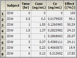
Part of the Semicompartmental Results worksheet

The Semicompartmental object generated four plots for each subject.

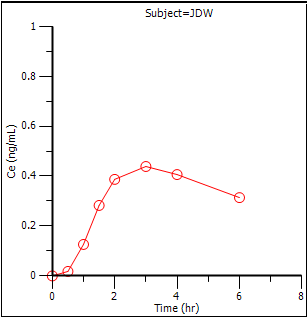
Effect-compartment concentration (Ce) over time (Ce vs Time)

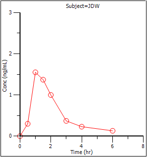
Concentration over time (Cp vs Time)

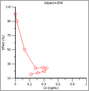
Effect as a function of Ce (Effect vs Ce)

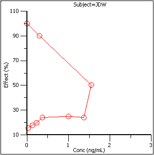
Effect over concentration (Effect vs Cp)

Based on the plots, PD model 103, an Inhibitory Effect E0 model, is appropriate to use to model the concentration in the effect compartment (Ce) versus effect relationship.

Model the pharmacodynamics

Right-click Workflow in the Object Browser and select New > Modeling > Least Squares Regression Models > PD Model.
Use the Select Source icon to map the Semicompartmental Results worksheet as the input source for the PD Model object.
In the Mappings panel:
Map Subject to the Sort context.
Leave Time mapped to None.
Leave Conc mapped None.
Map Ce to the X variable context.
Map Effect to the Y variable context.
In the Model Selection tab below the Setup panel, check the model Number 103 checkbox.

The default model parameter options are used. Phoenix generates initial parameter values and parameter bounds. To view the parameter option settings, select the Parameter Options tab.

Execute and view the PD Model results for the Semicompartmental output

Execute the object.

Phoenix analyzes each subject separately and includes all time points per subject.

The Final Parameters output provides estimates for E0 and IC50 for each subject. These are used later to predict steady-state effect values.

Click Observed Y and Predicted Y vs X under Plots.

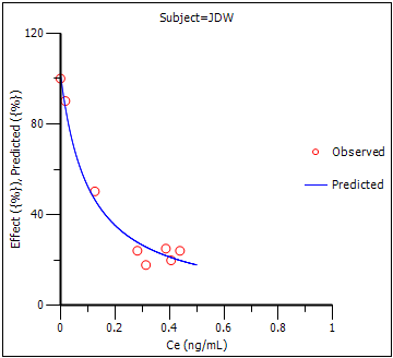
The Observed Y and Predicted Y vs X plot illustrates the fit of PD model 103 to the effect data when Ce from Semicompartmental modeling is used as the measure of exposure. The Observed Y and Predicted Y vs X plot for the first subject is shown below.

The other plots address model fit.

The NonParametric superposition example uses the output from this example. You may wish to save this project or leave the project open if you are continuing with the NonParametric superposition example.