NonParametric Superposition methodology
NonParametric superposition assumes that each dose of a drug acts independently of every other dose; that the rate and extent of absorption and average systemic clearance are the same for each dosing interval; and that linear pharmacokinetics apply, so that a change in dose during the multiple dosing regimen can be accommodated.
In order to predict the drug concentration resulting from multiple doses, one must have a complete characterization of the concentration-time profile after a single dose. That is, it is necessary to know C(ti) at sufficient time points ti, (i=1,2,…,n), to characterize the drug absorption and elimination process. Two assumptions about the data are required: independence of each dose effect, and linearity of the underlying pharmacokinetics. The former assumes that the effect of each dose can be separated from the effects of other doses. The latter, linear pharmacokinetics, assumes that changes in drug concentration will vary linearly with dose amount.
The required input data are the time, dosing, and drug concentration. The drug concentration at any particular time during multiple dosing is then predicted by simply adding the concentration values as shown in the next section (“Computation method”).
Note:User-defined terminal phases apply to all sort keys. In addition, dosing schedules and doses are the same for all sort keys.
Given the concentration data points C(ti) at times ti, (i=1,2,…,n), after a single dose D, one may obtain the concentration C(t) at any time t through interpolation if t1 < t <tn, or extrapolation if t > tn. The extrapolation assumes a log-linear elimination process; that is, the terminal phase in the plot of log(C(t)) versus t is approximately a straight line. If the absolute value of that line’s slope is lZ and the intercept is ln(b), then C(t) = bexp(–lZt) for (t > tn).
The slope lZ and the intercept are estimated by least squares from the terminal phase; the time range included in the terminal phase may be specified by the user or, if not specified, estimates from the best linear fit (based on adjusted R2 as in the Best Fit method in Noncompartmental Analysis) will be used. The half life is: ln(2)/lZ
Suppose there are m additional doses Dj, j = 1,…,m, and each dose is administered after t j time units from the first dose. The concentration due to dose Dj will be:
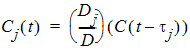
where t is time since the first dose and C(t – tj) = 0 for t £ tj.
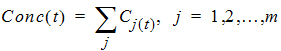
The total predicted concentration at time t will be:
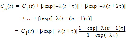
If the same dose is given at constant dosing intervals t, and t is sufficiently large that drug concentrations reflect the post-absorptive and post-distributive phase of the concentration-time profile, then steady state can be reached after sufficient time intervals. Let the concentration of the first dose be C1(t) for 0 < t < t, so t is greater than tn. Then the concentration at time t after nth dose (i.e., t is relative to dose time) will be:
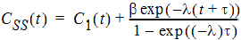
As  , the steady state (ss) is reached:
To display the concentration curve at steady state, Phoenix assumes steady state is at ten times the half life.
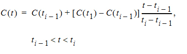
For interpolation, Phoenix offers two methods: linear interpolation and log-interpolation. Linear interpolation is appropriate for log-transformed concentration data and is calculated by:
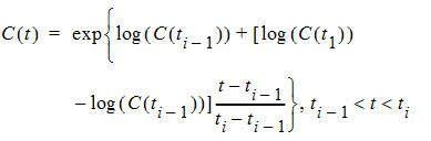
Log-interpolation is appropriate for original concentration data, and is evaluated by:
For additional information see Appendix E of Gibaldi and Perrier (1982). Pharmacokinetics, 2nd ed. Marcel Dekker, New York.
