Discrete and distributed delays

Transit compartment models, described by systems of ordinary differential equations (ODEs), have been widely used to describe delayed outcomes in pharmacokinetics and pharmacodynamics studies. The obvious disadvantage for this type of model is it requires manually finding proper values for the number of compartments, and hence it is time-consuming. It is also difficult, if not impossible, to do population analysis using this model. In addition, it may require many differential equations to fit the data and may not adequately describe some complex features.

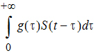
To alleviate these advantages, a distributed delay approach was proposed in “Hu, Dunlavey, Guzy, and Teuscher (2018)” to model delayed outcomes in pharmacokinetics and pharmacodynamics studies. It involves convolution of the signal to be delayed (S) and the probability density function (g) of the delay time,

Thus, for the distributed delay approach, the delay time may vary among signal mediators (e.g., drug molecules or cells), and hence it is a natural extension of the discrete delay approach that S(t – t) in which case, where the delay time is assumed to be the same (i.e., t) for all signal mediators.

Differential equations involving discrete delays and/or distributed delays are called delay differential equations (DDEs). The difference between ODEs and DDEs is that the future state of the system governed by ODEs is totally determined by its present value while for DDEs it is determined not only by its present value, but also by its past. This means that, for DDEs, one has to specify the values of the system state prior to the system starts (assuming throughout that the system starts at time zero). For example, for the following differential equation with a distributed delay,

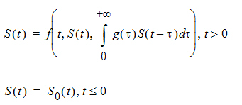
one has to specify the values of S(t) over all negative t; that is, one has to specify S₀, which is often called the history function.

It was shown in “Hu, Dunlavey, Guzy, and Teuscher (2018)” that the distributed delay approach is general enough to incorporate a wide array of pharmacokinetic and pharmacodynamic models as special cases, including transit compartment models, eﬀect compartment models, indirect response models with production either simulated or inhibited, typical absorption models (either zero-order or ﬁrst-order absorption), and a number of atypical (or irregular) absorption models (e.g., parallel ﬁrst-order, mixed ﬁrst-order, and zero-order, inverse Gaussian, and Weibull absorption models). This was done through assuming a speciﬁc distribution form for the delay time.

Speciﬁcally, transit compartment models are based on the assumption that the delay time is Erlang distributed, with shape and rate parameters respectively determining the number of transit compartments and the transition rate between the compartments. Note that Erlang distribution is a special case of the gamma distribution, which allows for non-integer shape parameters. Hence, distributed delay models with delay time assumed to be gamma distributed (referred to as gamma distributed delay models) are natural extension of transit compartment models. Examples for extending transit compartment models to their corresponding gamma distributed delay models can be found in “Hu, Dunlavey, Guzy, and Teuscher (2018)” and “Krzyzanski, Hu, and Dunlavey (2018)”.

The delay function

The delay function in PML can be used for both discrete delay and distributed delay (gamma, Weibull, and inverse Gaussian distribution are supported) and its syntax is given as follows:

delay(S, MeanDelayTime
     [, shape = ShapeParam]
    [, hist = HistExpression]
    [, dist = NameOfDistribution]
    )

If the shape option is not provided, then it describes a discrete delay and returns the value of:

S(t − MeanDelayTime)

Otherwise, it describes a distributed delay and returns the value of:

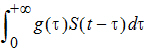
Here, g denotes the probability density function of the distribution specified in the dist option (whose value can be Gamma, Weibull, or InverseGaussian) with its shape parameter speciﬁed by the shape option and mean being MeanDelayTime. The hist option is used to specify the value of S prior to time 0; that is, if t < 0, then S(t)=HistExpression, which is required to be independent of time t, but can depend on variables that are defined at time 0 for the subject, such as covariates, ﬁxed and random eﬀects. If the hist option is not provided, then it is assumed that S(t)=0 for t < 0. If the dist option is not provided, then dist=Gamma is assumed.

It should be noted that the delay function relies on the fact that ODE solvers use shorter step sizes in the vicinity of rapid changes. Hence, it will not work in the presence of methods that have large step sizes, such as matrix exponent or closed-form. Even though there is no restriction on the number of delay functions put in a model, it should be used sparingly to avoid performance issue.

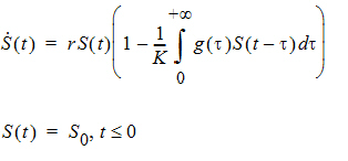
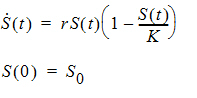
For the discrete delay function, the delay time can be estimated, and for the distributed delay case, both the mean and shape parameter for the specified distribution can be estimated. In addition, the delay function can be put on the right-hand side of a differential equation, and hence can be used to numerically solve a differential equation with either discrete delays or distributed delays, no matter whether the signal to be delayed, S, depends on model states or not. For example, the delay function can be used to numerically solve the well-known Hutchinson equation (a logistic growth model with a discrete delay):

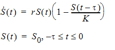
where r denotes the intrinsic growth rate, K is the carrying capacity, and S₀ is a positive constant. The PML code for this model is given as follows:

deriv(S=r*S*(1-delay(S, tau, hist=S0)/K))
sequence{S=S0}

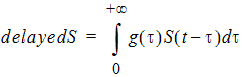
The delay function can also be used to numerically solve the following logistic growth model with a distributed delay:

where g is the probability distribution function of the supported distribution (gamma, Weibull, or inverse Gaussian) with shape parameter being ShapeParam and mean being MeanDelayTime. The PML code for this model with a Weibull distributed delay is given as follows:

delayedS = delay(S, MeanDelayTime,
     shape = ShapeParam,
     hist = S0,
    dist = Weibull
     )
deriv(S = r*S*(1-delayedS/K))
sequence{S = S0}

A simple simulation of the logistic growth model with a gamma distributed delay (the previous equation) is given in example project LogisticGrowthModelWithGammaDistributedDelay.phxproj (located in …\Examples\NLME). The project demonstrates that the previous equation can exhibit much richer dynamics than its corresponding ODE.

For example, it may produce an oscillation around the carrying capacity while the corresponding ODE cannot. In addition, adjusting the mean delay time can achieve the desired type of oscillations (either damped or sustained oscillations).

The delayInfCpt statement

Note that, the signal to be delayed, S, in the delay function cannot contain dosing information from the input data set. Hence, it cannot be used for the absorption delay case. To achieve this, a compartment modeling statement, delayInfCpt, was added to PML with its syntax given as follows:

delayInfCpt(A, MeanDelayTime,
    ParamRelatedToShape
    [, in = inflow]
    [, out = outflow]
    [, dist = NameOfDistribution]
    )

Here, A denotes a compartment that can receive doses (from the input data set) through the dosepoint statement. The second and third arguments are used to characterize the distribution specified in the dist option, which has values of Gamma, Weibull, and InverseGaussian. Specifically, the second argument denotes the mean of the specified distribution, and the third argument is related to the shape parameter of the specified distribution:

•If dist = InverseGaussian, then ParamRelatedToShape = ShapeParameter,

•Otherwise, ParamRelatedToShape is set to be ParamRelatedToShape = ShapeParameter–1, and it must be non-negative so as to prevent the shape parameter from being less than one (which causes a singularity of the probability density function of the gamma or Weibull distribution at time 0).

The optional in option is used to specify any additional flow that is delayed with its history function assumed to be zero. The optional out option is used to specify flow rates (either out of or into compartment A) that are not delayed. If the dist option is not provided, then the system automatically assumes that dist = Gamma.

Mathematically, the delayInfCpt statement means:

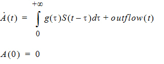
Here S denotes all the input to be delayed, including the dose and the inﬂow speciﬁed by the in option, with S(t)=0 if t < 0, and g is the probability distribution function of the distribution specified by the dist option. The outﬂow is defined by the out option.

There are two examples that demonstrate how to use delayInfCpt to model absorption delay. For the ﬁrst one, the delay time between the administration time of the drug and the time when the drug molecules reach the central compartment is assumed to be gamma distributed with the mean given by MeanDelayTime and shape parameter ν given by ν=ShapeParamMinusOne+1. In addition, the drug is assumed to be described by a one-compartment model with a ﬁrst-order clearance rate. The PML code for the structure model of this example is then given by:

# central compartment
delayInfCpt(A1, MeanDelayTime,
     ShapeParamMinusOne,
     out =-Cl*C
     )
dosepoint(A1)
# drug concentration at the central compartment
C=A1/V

The second example is about double sites of absorption, where the drug is assumed to be described by a two-compartment model with a ﬁrst-order elimination from the central compartment. In addition, the delay time between the administration time of the drug and the time when the drug molecules reach the central compartment is assumed to be gamma distributed for each pathway. The PML code for the structure model of this example is then given by:

# 1st pathway contribution to the central compartment,
# where frac denotes the fraction of dose absorbed by
# the 1st pathway, and the remaining dose is
# absorbed by the 2nd pathway.
delayInfCpt(Ac1, MeanDelayTime1, ShapeParamMinusOne1,
out=-Cl*C-Cl2*(C-C2)
)
dosepoint(Ac1, bioavail=frac)
# 2nd pathway contribution to the central compartment
delayInfCpt(Ac2, MeanDelayTime2, ShapeParamMinusOne2)
dosepoint(Ac2, bioavail=1-frac)
# Peripheral compartment
deriv(A2=Cl2*(C-C2))
# Drug concentration at the central compartment
C=(Ac1+Ac2)/V
# Drug concentration at the peripheral compartment
C2=A2/V2

The model ﬁtting for the first example (called gamma absorption delay model) is demonstrated in the example project ModelAbsorptionDelay_delayInfCpt.phxproj (located in …\Examples\NLME). In the project, there are two other models that are exactly the same as the gamma absorption delay model, but with the absorption delay time assumed to be either inverse Gaussian distributed (called inverse Gaussian absorption delay model) or Weibull distributed (called Weibull absorption delay model). The estimation results obtained for these three models show that the shape parameter and the mean delay time can be reliably estimated along with the other parameters. In addition, standard diagnostic plots are good.

The Model Comparer tool is then used to compare these three models and shows that the gamma absorption delay model is the best one to describe the given data (in terms of having a lower AIC/BIC value), see the workflow ModelComparer in the project for details. The visual predictive check (VPC) is then performed for the gamma absorption delay model with initial estimates for Theta, sigma, and Omega set to their corresponding final estimates (by using the Accept All Fixed+Random button in the Parameters > Fixed Effects sub-tab to accept the final parameter estimates as the initial estimates), see the workflow VPC in the project for details. The VPC plots suggest that the gamma absorption delay model provides a reasonably good explanation of the data.

The gammaDelay statement

PML provides an alternative function, gammaDelay, to describe a gamma distributed delay. The difference between the gammaDelay function and the delay function with dist = Gamma is how the integral is approximated. The delay function involves direct numerical calculation of the integral with the values of the signal to be delayed recorded in a table upon every derivative evaluation and, hence, it may become very expensive or even prohibitive for complex population analysis. The gammaDelay function, on the other hand, is based on the ODE approximation method provided in Krzyzanski, 2019, wherein it was shown that this approach is much faster than the delay function.

The syntax of the gammaDelay function is given as follows:

gammaDelay(S, MeanDelayTime
    , shape = ShapeParam
    [, hist = HistExpression]
    , numODE = NumberOfODEUsed
    )

Here S denotes the signal to be delayed. The second argument denotes the mean for the gamma distribution. The shape option must be provided and it is used to specify the shape parameter of the gamma distribution. The hist option is used to specify the value of S prior to time 0. If this option is not provided, then it is automatically assumed that S(t)=0 for t<0. The numODE option must be provided and it is used to specify the number of ODEs used to approximate the integral. The maximum number of ODEs allowed is 400.

The accuracy of the approximation for the gammaDelay function depends on the number of ODEs used: the higher the number of ODEs used, the more accurate the approximation. However, the performance cost increases as the number of ODEs increases. In addition, a large number of ODEs may lead to numerical difficulties in the ODE solver. Hence, some exploratory analysis of the effect of number of ODEs on the solution of the given problem is recommended. Here is a general guideline, given in Krzyzanski, 2019, on the number of ODEs used: if the shape parameter for the gamma distribution is greater than one, then at least 21 ODEs are needed; otherwise, more than 101 ODEs are needed.

The gammaDelay function can also be put on the right-hand side of a differential equation. In addition, the mean and shape parameter for the gamma distribution can be estimated. The example project OneCpt0OrderAbsorp_gammaDelayEmax.phxproj (located in …\Examples\NLME) demonstrates how to use the gammaDelay function to describe a delayed drug response given below:

Here g is the probability density function of a gamma distribution with mean being MeanDelayTime and shape parameter being ShapeParam, and S is described by an Emax model:

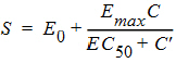
where the drug concentration, C, is described by a one-compartment model with zero-order absorption and first-order elimination. Note that C(t) = 0 for t £ 0. Hence S(t) = E₀ for t £ 0. Thus the PML code for the delayed drug response is given as follows:

delayedS = gammaDelay(S, MeanDelayTime
    , shape = ShapeParam
    , hist = E0
    , numODE = 21
    )

where the value of numODE is chosen based on some exploratory analysis (see the workflow Effect_NumODE_Solution in the project, which shows that the solutions obtained using 21 ODEs are similar to ones obtained using 41 or 81 ODEs). The model fitting results (given in the workflow Estimation) show that the shape parameter and the mean delay time can be reliably estimated along with the other parameters, and that standard diagnostic plots are reasonably good.

References

Hu, Dunlavey, Guzy, and Teuscher (2018)

A distributed delay approach for modeling delayed outcomes in pharmacokinetics and pharmacodynamics studies. J Pharmacokinet Pharmacodyn. https://doi.org/10.1007/s10928-018-9570-4.

Krzyzanski, Hu, and Dunlavey (2018)

Evaluation of performance of distributed delay model for chemotherapy-induced myelosuppression. J Pharmacokinet Pharmacodyn. https://doi.org/10.1007/s10928-018-9575-z.

Krzyzanski (2019)

Ordinary differential equation approximation of gamma distributed delay model. J Pharmacokinet Pharmacodyn. https://doi.org/10.1007/s10928-018-09618-z.