Perhaps the most common application of deconvolution is in the evaluation of drug release and drug absorption from orally administered drug formulations. In this case, the bioavailability is evaluated if the reference input is a vascular drug input. Similarly, gastrointestinal release is evaluated if the reference is an oral solution (oral bolus input). Both are included here.
This example uses the dataset M3tablet.dat, which is located in the Phoenix examples directory. The analysis objectives are to estimate the following for a tablet formulation:
Knowledge of how to do basic tasks using the Phoenix interface, such as creating a project and importing data, is assumed.
•Absolute bioavailability and rate and cumulative extent of absorption over time (see “Evaluate absolute bioavailability”)
•In vivo dissolution and the rate and cumulative extent of release over time (see “Estimate dissolution”)
The completed project (Deconvolution.phxproj) is available for reference in …\Examples\WinNonlin.
Evaluate absolute bioavailability
To estimate the absolute bioavailability, the mean unit impulse response parameters A and alpha have already been estimated from concentration-time data following instantaneous input (IV bolus) for three subjects, using PK model 1. The data in M3tablet.dat includes those parameter estimates and plasma drug concentrations following oral administration of a tablet formulation. This example shows how to estimate the rate at which the drug reaches the systemic circulation, using deconvolution.
For this type of data, all the data for one treatment must be displayed in the first rows, followed by all the data for the other treatment.
-
Create a project called Deconvolution.
-
Import the file …\Examples\WinNonlin\Supporting files\M3tablet.dat.
-
Right-click M3tablet in the Data folder and select Send To > Computation Tools > Deconvolution.
-
In the Main Mappings panel:
Map subject to the Sort context.
Leave time mapped to the Time context.
Map conc to the Concentration context.
Leave all the other data types mapped to None. -
Select Exp Terms in the Setup list.
-
Select the Use Internal Worksheet checkbox.
-
In the Value column type 100 for each row with A1 in the Parameter column.
-
In the Value column type 0.98 for each row with Alpha1 in the Parameter column.
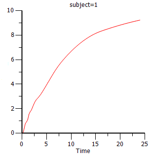
There are no dose amounts for this example. The calculated fractional input approaches a value of 1 rather than being adjusted for dose amount. -
Click
 (Execute icon) to execute the object.
Phoenix generates worksheets and plots for the output. Partial results for subject 1 are displayed below. -
Select Cumulative Input Plot in the Results list.
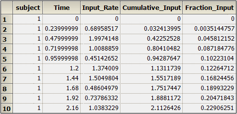
Part of the Values worksheet
To estimate the in vivo dissolution from the tablet formulation, the mean unit impulse response parameters A and alpha have already been estimated from concentration-time data following instantaneous input into the gastrointestinal tract by administration of a solution, using PK model 3. The steps below show how to use deconvolution to estimate the rate at which the drug dissolves.
For the rest of this example an oral solution (oral bolus) is used to estimate the unit impulse response. In this case, the deconvolution result should be interpreted as an in vivo dissolution profile, not as an absorption profile. The oral impulse response function should have the property of the initial value being equal to zero, which implies that the sum of the ‘A’s must be zero. The alphas should all still be positive, but at least one A will be negative.
-
Right-click M3tablet in the Data folder and select Send To > Computation Tools > Deconvolution.
-
In the Main Mappings panel:
Map subject to the Sort context.
Leave time mapped to the Time context.
Map conc to the Concentration context.
Leave all the other data types mapped to None. -
In the Options tab below the Setup panel, select 2 in the Exponential Terms menu.
-
Select Exp Terms in the Setup list.
-
Check the Use Internal Worksheet checkbox.
-
Fill in the Value column as follows:
Type -110 for each row with A1 in the Parameter column.
Type 110 for each row with A2 in the Parameter column.
Type 3.8 for each row with Alpha1 in the Parameter column.
Type 0.10 for each row with Alpha2 in the Parameter column. -
Execute the object.
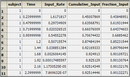
Results for subject 1 are displayed below: -
Select Cumulative Input Plot under Plots in the Results list.
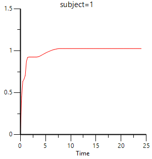
This concludes the Deconvolution example.
