Phoenix’s Crossover object performs statistical analysis of data arising from subjects when variance homogeneity and normality may not necessarily apply. This tool performs nonparametric statistical tests on variables such as Tmax and provides two categories of results. First, it calculates intervals for each treatment median. It then calculates the median difference between treatments and the corresponding intervals. Finally, it estimates the relevance of direct, residual, and period effects.
Use one of the following to add the object to a Workflow:
Right-click menu for a Workflow object: New > Computation Tools > Crossover.
Main menu: Insert > Computation Tools > Crossover.
Right-click menu for a worksheet: Send To > Computation Tools > Crossover.
Note:To view the object in its own window, select it in the Object Browser and double-click it or press ENTER. All instructions for setting up and execution are the same whether the object is viewed in its own window or in Phoenix view.
Main Mappings panel
Options tab
Results
Crossover methodology
Data and assumptions
References
Crossover design example
For a brief description of datasets used with the Crossover object, see “Data and assumptions”.
Use the Main Mappings panel to identify how input variables are used in a Crossover object. The mapping options in the Main Mappings panel change depending on whether the dataset used with the object contains treatment data in a stacked or separate layout. Required input is highlighted orange in the interface.
None: Data types mapped to this context are not included in any analysis or output.
Sort: Categorical variable(s) identifying individual data profiles, such as subject ID and treatment in a crossover study. A separate analysis is performed for each unique combination of sort variable values.
Subject: The subjects in a dataset.
Sequence: The order of drug formulation administration.
Stacked Treatment Data
Response: The measured response to a drug formulation.
Treatment: The treatment drug formulations used in a study, presented in a stacked format.
Separated Treatment Data
Test Treatment: The treatment drug formulation being tested in a study.
Reference Treatment: The treatment drug formulation used as a reference in a study.
-
In the Treatment Data Layout menu, select the method used to store treatment data in a dataset.
Stacked: The drug formulations are arranged in the same column in a dataset.
Separate: The drug formulations are separated into two columns in a dataset, Test and Reference. -
In the Reference Treatment menu, select the treatment to serve as the reference. Available for stacked data only.
The Crossover object creates two worksheets and one text file in the Results tab. The worksheets are called Confidence Intervals and Effects. The text file is called Settings.
The Confidence Intervals worksheet lists the intervals at 80%, 90%, and 95% for the treatment medians in the crossover data and the treatment difference median.
The Effects worksheet lists the test statistic and p-value associated with each of four tests. It includes tests for an effect of sequence, treatment and period, as well as treatment and residual simultaneously.
The Settings text file lists the user-specified settings in the Crossover object.
Units associated with the Response variable in the input dataset units are carried through to the Crossover object output. The output worksheets display units in the median, lower, and upper value parameters.
The two-period crossover design is common for clinical trials in which each subject serves as his or her own control. In many situations the assumptions of variance homogeneity and normality, relied upon in parametric analyses, may not be justified due to small sample size, among other reasons. The nonparametric methods proposed by Koch (1972) (The use of nonparametric methods in the statistical analysis of the two-period change-over design. Biometrics 577–83.) can be used to analyze such data.
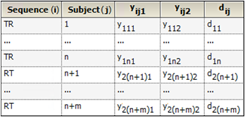
Consider a trial testing the effects of two treatments, Test (T) and Reference (R). Suppose that n subjects are randomly assigned to the first sequence, TR, in which subjects are given treatment T first and then treatment R following an adequate washout period. Similarly, m subjects are assigned to the RT sequence. Y represents the outcome of the trial (for example Cmax or Tmax) and yijk is the value observed on sequence i (i=1,2), subject j (j = 1,2,…,n, n+1,…n+m) and period k (k=1,2). Treatment is implied by sequence i and period k, for example i=1 and k=1 is treatment T; i=1 and k=2 is treatment R. The data are listed in columns 1 through 4 of the following table, and column 5 gives the within-subject difference in Y between the two periods, where:
dij = yij1 – yij2

Then the n*m crossover differences (d1i – d2j)/2 are computed, along with the median of these n*m points. This median is the Hodges-Lehmann estimate of the difference between the median for T and the median for R.
Crossover Design supports two data layouts: stacked in same column or separate columns. For “stacked” data, all measurements appear in a single column, with one or more additional columns flagging which data belong to which treatment. The data for one treatment must be listed first, then all the data for the other. The alternative is to place data for each treatment in a separate column.
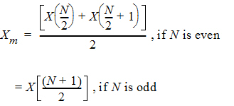
The median response and its interval are calculated for Y of each treatment and the crossover difference between treatments, C. Let X(1), X(2),…, X(N) be the order statistic of samples X1, X2,…, XN. The median Xm is defined as:

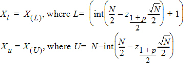
The 100% confidence interval (CI) of Xm is defined as follows.
•For N <= 20, the exact probability value is obtained from a Mann-Whitney U-distribution.
•For N > 20, normal approximation is used:

where int(X) returns the largest integer less than or equal to X.
Four hypotheses are of interest:
•no sequence effect (or drug residual effect);
•no treatment effect given no sequence effect;
•no period effect given no sequence effect; and
•no treatment and no sequence effect.
Hypothesis 1 above can be tested using the Wilcoxon statistic on the sum S. If R(Sl) is the rank of Sij in the whole sample, l = 1,…, n+m. The test statistic is:

The p-value is evaluated by using normal approximation (Conover, 1980):

Similarly, hypothesis 2 can be tested using the Wilcoxon statistic on the difference D; hypothesis 3 can be tested using the Wilcoxon statistic on the crossover difference C. The statistics are in the form described above.
Hypothesis 4 can be tested using the bivariate Wilcoxon statistic on (Yij1, Yij2). For each period k, let Rijk equal:

The average rank for each sequence is:

where j=1,…, ni, ni=n for i=1, and ni=m for i=2
Thus, the statistic to be used for testing hypothesis 4 is:

where Ui is a 2x1 vector:

S is the 2x2 covariance matrix:

and L ~ X2, so the p-value can be evaluated.
Conover (1980). Practical Nonparametric Statistics 2nd ed. John Wiley & Sons, New York.
Dixon and Massey (1969). Introduction to Statistical Analysis, 3rd ed. McGraw-Hill Book Company, New York.
Koch (1972). The use of non-parametric methods in the statistical analysis of the two-period change-over design. Biometrics 577–84.
Kutner (1974). Hypothesis testing in linear models (Eisenhart Model 1). The American Statistician, 28(3):98–100.
Searle (1971). Linear Models. John Wiley & Sons, New York.
Steel and Torrie (1980). Principles and Procedures of Statistics; A Biometrical Approach, 2nd ed. McGraw-Hill Book Company, New York.
Winer (1971). Statistical Principles in Experimental Design, 2nd ed. McGraw-Hill Book Company, New York, et al.
