Using a number of the sample files provided with the Phoenix software, this tutorial introduces the steps to complete the following common tasks:
Most Phoenix objects require the same basic steps for their use. However, there may be multiple paths to accomplishing a step (e.g., main menu, right-click menu, drag-and-drop, etc.). For simplicity, only one is listed here.
Note:Any object added to a project can be viewed in its own window by selecting the object in the Object Browser and double-clicking it or pressing ENTER. All instructions for setting up and executing an object are the same whether the object is viewed in its own window or in Phoenix’s viewing.
Start Phoenix and create a new project
-
Double-click the Phoenix icon (
 ) on your desktop to start Phoenix.
 -
Select File > New Project to create a new project.
A new project is created in the Object Browser and is in edit mode for you to name. -
Name the new project by typing Quick Tour.
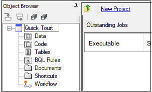
The left panel’s default view is the Object Browser, which contains the project, and the other folders and objects that are contained in the project. The right viewing panel’s default view is blank, unless one of the project folders or the workflow is selected.
Import a dataset
The dataset Bguide1.dat is used to test key Phoenix functions.
-
Select File > Import or click
 .
. -
Navigate to <Phoenix_install_dir>\application\Examples\WinNonlin\Supporting files).
-
Select the file Bguide1.dat and click Open.
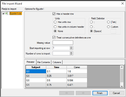
The File Import Wizard dialog is displayed. The dialog is used to assign options for how the data are imported and presented. -
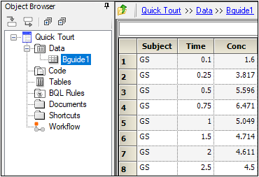
Click Finish. The dataset is added to the project Data folder and the worksheet is displayed in the right viewing panel.
Create a plot
-
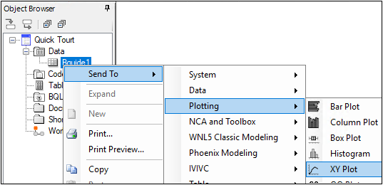
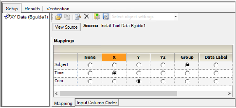
Right-click Bguide1 in the Data folder and select Send To > Plotting > XY Plot from the menu.
-
Use the option buttons in the XY Data Mappings panel to map the data types to the following contexts:
Map Subject to the Group context.
Map Time to the X context.
Map Conc to the Y context. -
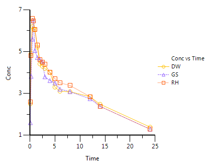
Click
 to execute the workflow.
 -
Now use the Bguide1 dataset to test the Table object and its summary statistics function.
An XY Plot object can also be added to a Workflow by selecting the Workflow object in the Object Browser and then selecting Insert > Plotting > XY Plot.
Or right-clicking the Workflow object and selecting New > Plotting > XY Plot and then using the pointer to drag the Bguide1 worksheet from the Data folder to the XY Data Mappings panel.
The default view of an object is the Setup tab, which contains all the steps necessary to set up an object.
Create a table
-
Right-click Bguide1 in the Data folder and select Send To > Table > Table from the menu.
-
Use the option buttons in the Main Mappings panel to map the data types to the following contexts:
Map Subject to the Stratification Row context.
Leave Time mapped to None.
Map Conc to the Data context.
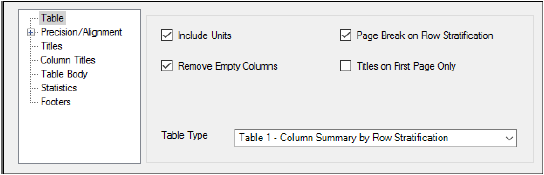
Use the Options tab to specify which table type the Table object uses. The Options tab is located below the Setup tab. -
In the Table Type menu, select Table 1 - Column Summary by Row Stratification.
-
Select the Page Break on Row Stratification checkbox.
-
Select the Statistics tab, which is located underneath the Setup tab.
-
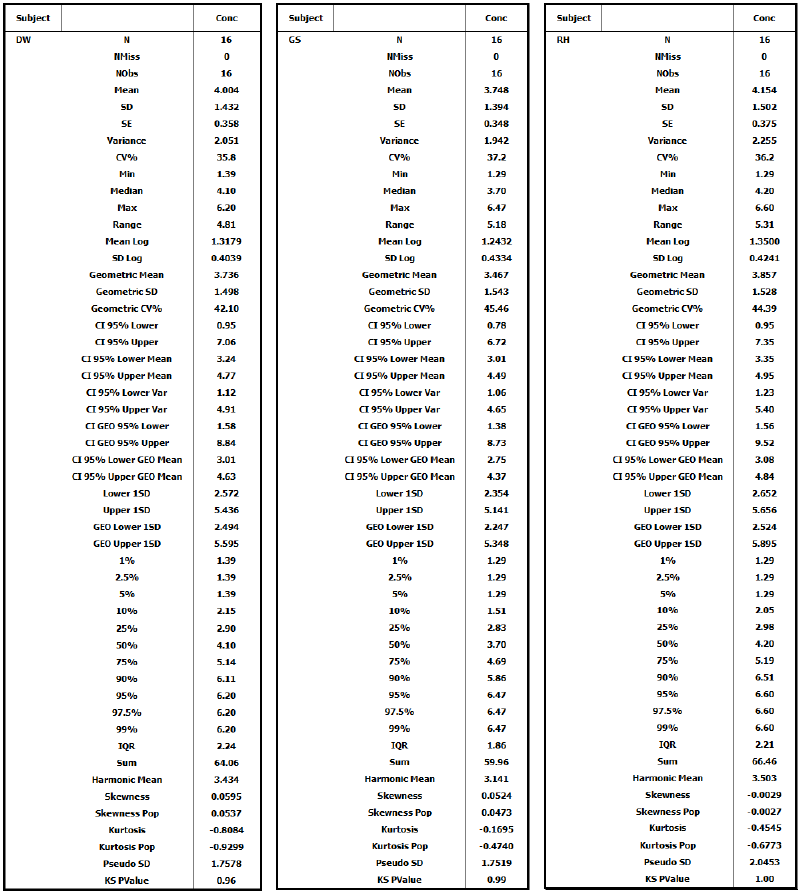
Click Select All to select all output statistics.
-
Click
 .
.
The results are presented as three HTML tables in the Results tab. Compare the tables in the Results tab to the tables pictured below.
Execute noncompartmental analysis
-
Select File > Load Project. The Load Project dialog is displayed.
-
Navigate to <Phoenix_install_dir>\application\Examples\WinNonlin.
-
Select Multiple_Profiles.phxproj and click Open.
This project contains:
– A dataset worksheet (profiles)
– A worksheet of dosing information (Dosing published from NCA)
– An XY Plot object
– An NCA model object
– A Descriptive Stats object
– A Data Wizard object
– An XY Plot (X-Categorical) object -
Expand the workflow node.
-
Select the NCA model object in the Object Browser.
-
Select items in the Setup tab list to explore the data mappings and option settings.
-
Click
 to execute the object.
Text output
The Core output contains the model settings and the same data as the worksheets, but presented in plain ASCII text. If there were errors in the model they would be listed here. Below is part of a Core output text file.
...
Model: Plasma Data, Extravascular Administration
Number of nonmissing observations: 12
Dose time: 0.00
Dose amount: 100.00
Calculation method: Linear Trapezoidal with Linear Interpolation
Weighting for lambda_z calculations: Uniform weighting
Lambda_z method: Find best fit for lambda_z, Log regression
Compute Concentrations at: 75
Summary Table
-------------
Time Conc. Pred. Residual AUC AUMC Weight
min ng/ml ng/ml ng/ml min*ng/ml min*min*ng/ml
------------------------------------------------------------
0.0000 0.0000 0.0000 0.0000
5.000 340.3 850.8 4254.
10.00 1914. 6487. 5.636e+04
15.00 2069. 1.644e+04 1.818e+05
20.00 1471. 2.529e+04 3.329e+05
30.00 788.8 3.659e+04 5.983e+05
45.00* 496.4 460.9 35.54 4.623e+04 9.434e+05 1.000
60.00* 372.8 357.2 15.63 5.275e+04 1.279e+06 1.000
90.00* 204.3 214.6 -10.33 6.141e+04 1.890e+06 1.000
120.0* 124.1 128.9 -4.852 6.633e+04 2.389e+06 1.000
180.0* 39.25 46.52 -7.266 7.123e+04 3.048e+06 1.000
240.0* 19.32 16.79 2.531 7.299e+04 3.399e+06 1.000
The Settings file lists all the settings used to specify the noncompartmental analysis. Below is part of a Settings text file.
...
Sort: Subject, Form
Time: Time [min]
Concentration: Conc [ng/mL]
Carry:
Dosing: (Internal)
Slopes: (Internal)
Partial Areas: (Internal)
Therapeutic Response: <None>
Units: (Internal)
Parameter Names: <None>
...
Plasma Model
Title=Processing Multiple Profiles with Model 200
Linear Trapezoidal Linear Interpolation
Sparse=False
Weighting=Uniform Weighting; 0
Dose Type=Extravascular
Dose Unit=ng
Dose Normalization=None
Compute Concentrations at: 75
Output data
The NCA object creates seven results worksheets: Dosing Used, Exclusions, Final Parameters, Final Parameters Pivoted, Partial Areas, Plot Titles, Slopes Settings, and Summary Table. Selections from the Final Parameters and Summary Table worksheets are shown below.
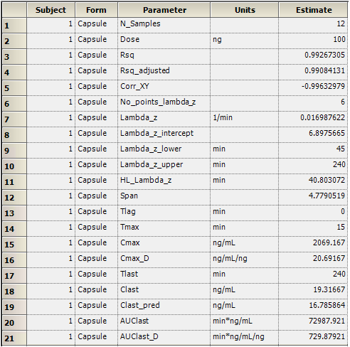
Part of the Final Parameters worksheet
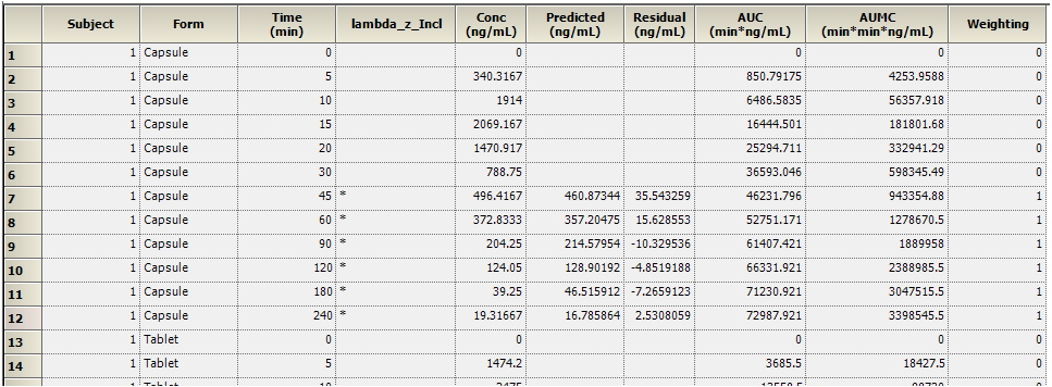
Part of the Summary Table worksheet
A total of 12 plots are generated; one for each of two formulations, for each of the six subjects. The first two charts for subject one are shown below.
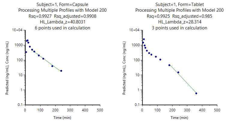
Plots for subject one, capsule and tablet formulation
Perform pharmacokinetic modeling
-
Select File > Load Project. The Load Project dialog is displayed.
-
Navigate to <Phoenix_install_dir>\application\Examples\WinNonlin.
-
Select PK_Model.phxproj and click Open.
This project contains:
– A dataset worksheet (study1)
– An XY Plot object
– A PK model object -
Expand the workflow node.
-
Select the PK Model object in the Object Browser.
-
Select items in the Setup tab list to explore the model’s data mappings and option settings.
The imported PK Model object uses PK Model 3, which is a one-compartment model with 1st order absorption. -
Click
 to execute the object.
Worksheet results
The PK Model object’s output worksheets partially include Condition Numbers, Diagnostics, Dosing Used, Final Parameters, Initial Estimates, Secondary Parameters, and Summary Table. The Final Parameters, Secondary Parameters, and Summary Table worksheets are shown below.

Final Parameters worksheet
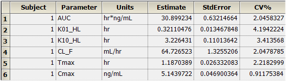
Secondary Parameters worksheet
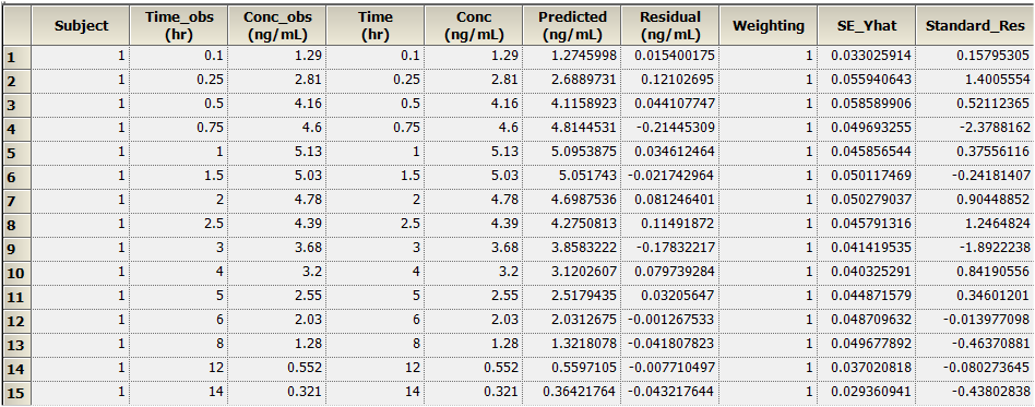
Summary Table worksheet
Text output
The Core output text results include all model settings and iterations, including the output from the worksheets. Any model errors would be listed here. Below is part of the Core output text file.
...
Listing of input commands
MODEL 3
NVAR 3
NPOI 1000
XNUM 2
YNUM 3
NCON 3
CONS 1,2,0
METH 2'Gauss-Newton (Levenberg and Hartley)
ITER 50
INIT 0.25,1.81,0.23
MISS '.'
DATA 'WINNLIN.DAT'
BEGIN
The Settings file lists all the settings used to specify the noncompartmental analysis. Below is part of the Settings text file.
...
Main: PK Model.Data.study1
Sort: Subject
Time: Time [hr]
Concentration: Conc [ng/mL]
Carry:
Dosing: (Internal)
Initial Estimates: (Internal)
Units: (Internal)
***** Other Parameters *****
...
PK 3-[PK]
Gauss-Newton (Levenberg and Hartley)
Convergence criteria of 0.0001 used during minimization process
50 maximum iterations allowed during minimization process
Plots
The plot results include Observed Y and Predicted Y vs X, Partial Derivatives Plot, Predicted Y vs Observed Y, Predicted Y vs X, Residual Y vs Predicted Y, and Residual Y vs X. Some plot results are shown below.
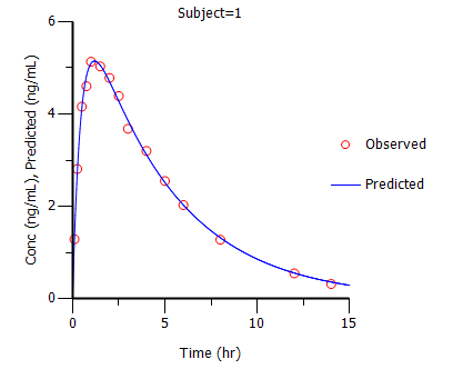
Observed Y and Predicted Y vs X
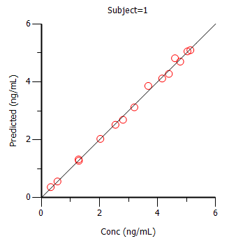
Predicted Y vs Observed Y
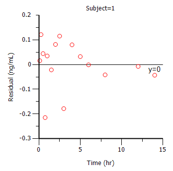
Residual Y vs X
Execute a bioequivalence model
-
Select the Install Test project in the Object Browser.
-
Select File > Import.
-
In the Import File(s) dialog, navigate to <Phoenix_install_dir>\application\Examples\Supporting files.
-
Select the file Seq2Per4.csv and click Open.
In the File Import Wizard dialog, click Finish. The dataset is added to the project Data folder. -
Select the project workflow in the Object Browser and then select Insert > NCA and Toolbox > Bioequivalence.
The Bioequivalence object is added to the workflow in the Object Browser. -
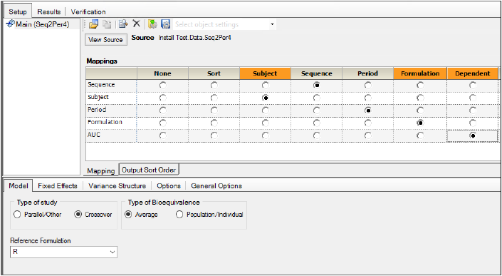
Use the pointer to drag the Seq2Per4 worksheet from the Data folder to the Main Mappings panel.
The Seq2Per4 dataset is mapped to the Bioequivalence object. -
Use the option button in the Main Mappings panel to map AUC to the Dependent context.
The following data types are automatically mapped to contexts when the dataset is mapped to the Bioequivalence model.
– Sequence is mapped to the Sequence context.
– Subject is mapped to the Subject context.
– Period is mapped to the Period context.
– Formulation is mapped to the Formulation context.
– AUC is mapped to the Dependent context. -
In the Model tab (located below the Setup tab), ensure that Crossover is selected as the Type of study, Average is selected as the Type of Bioequivalence, and R is selected as the Reference Formulation.
-
Select the Fixed Effects tab, which is located underneath the Setup tab.
-
Ln(x) is automatically selected in the Dependent Variables Transformation menu. Do not change this setting.
-
Click
 to execute the object.
Note:The default settings for a new Bioequivalence model are Crossover as the type of study and Average as the type of bioequivalence.
Output data
The bioequivalence model worksheet output partially includes Average Bioequivalence, Diagnostics, Final Fixed Parameters, Final and Initial Variance Parameters, Least Squares Means, and Sequential Tests. The Diagnostics, Final Variance Parameters, and Sequential Tests worksheets are shown below.


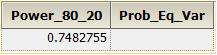
Average Bioequivalence worksheet
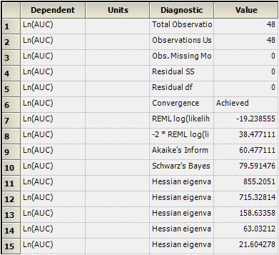
Diagnostics worksheet
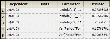
Final Variance Parameters worksheet
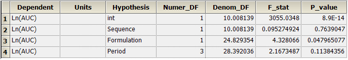
Sequential Tests worksheet
This concludes the Quick Tour of Phoenix.
