The following example demonstrates the syntax for defining a population PK model.
1 mymodel(){
2 ## STRUCTURAL MODEL SECTION
3 deriv(aa=-aa*ka)
4 deriv(a1=aa*ka-a1*cl/v)
5 dosepoint(aa)
6 c=a1/v
7 ## PARAMETER MODEL SECTION
8 stparm(
9 ka=tvKa*exp(nKa)
10 cl=tvCl*exp(nCl)
11 v=tvV*exp(nV)
12 )
13 fixef(
14 tvKa=c(, 10,)
15 tvCl=c(, 5,)
16 tvV=c(, 8,)
17 )
18 ranef(
19 diag(nKa, nCl, nV)=c(1.0, 0.5, 0.6)
20 )
21 ## ERROR MODEL SECTION
22 error(eps1=0.01)
23 observe(cObs=c+eps1)
24 }
Lines 1–24 define a model called “mymodel.” It is a one-compartment, first-order model parameterized by clearance and volume. The model statements can be roughly grouped into sections for structural, parameter, and error models. The model contains several user-defined and reserved names.
Line 3 gives the differential equation for the absorption compartment. It is read as “the derivative of aa is -aa*ka.” The variable aa represents the amount of the drug in the absorption compartment.
Line 4 gives the differential equation for amount in the central compartment, a1.
Note:PML works best when the right-hand-side of each differential equation has no time-discontinuities. An example of a system which is time-discontinuous is:
deriv (a1=-a1*cl/v)
cl=(t<t1 ? cl1:cl2)
This is time-discontinuous because clearance jumps at time t1 from cl1 to cl2 and it appears on the right-hand-side of the differential equation for a1. This has the effect of causing the ODE solver to step back and forth over time t1, in ever smaller steps, attempting to reduce its error. It is much better to use the sequence statement (explained below), which can run the ODE solver up to particular times (called change points), then perform some discontinuous modifications to the model and run the ODE solver forward again. In fact, if Matrix Exponent is requested, it will not run this code. It will switch to a different solver, because it requires that the system be not only continuous, but linear between change points. See “Matrix Exponent” for more information about this method.
The use of t, representing time since the subject began processing, is discouraged, because it is most often used in the above manner.
Line 5, the dosepoint statement, says that aa, the absorption compartment, can receive doses. If the central compartment can also take doses, the model can include an additional dosepoint statement.
Line 6 is a simple assignment statement saying that concentration c in the central compartment is equal to the amount in the central compartment a1 divided by volume v. This quantity is related to the observed quantity in line 23.
Lines 8–12 identify the structural parameters and their associations with the fixed and random effects. If a model is used for single-subject estimation, only the fixed effects are estimated. The model can include any number of stparm statements. Structural parameter statements should only include fixed effects, random effects, and covariates. They should not include variables that are evaluated as assignment statements. Structural parameter statements are executed before anything else and are only re-executed during a given iteration if a covariate changes, so any variables from assignment statements will be undefined on the initial execution of the stparm statements, possibly leading to model failure.
Lines 13–17 identify the population fixed effect parameters (thetas). It is recommended that a consistent naming convention is used to make the model more easily understood by others. In this example, variables representing typical values start with the letters “tv,” followed by a capitalized variable name, such as tvCl for clearance or tvV for volume. The model can include any number of fixed effect statements.
After each fixed effect is an optional assignment, providing either a single number representing the initial value of the parameter or a list of three numbers representing a lower bound, an initial value, and an upper bound, in that order.
If the assignment is used, then the initial estimate must be provided. The lower and upper bound values can be omitted, but the order must be maintained by using blank spaces and commas as delimiters. The correct syntax is:
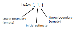
If one value is provided it is assumed that the lower and upper boundaries are not being supplied, but the syntax must be correct. For example, tvA=c(1) does not work. However, users can omit the parenthesis and use tvA=1, and the PML assumes that one is the initial value assigned to the parameter.
Lines 18–20 identify the random effects (etas). In this model, there are three random effect variables grouped into a single block, which causes a diagonal omega matrix to be estimated. The initial value of the omega matrix is given as a list of numbers. Multiple blocks are supported. The model can include any number of ranef statements.
Assignment statements are performed in the order that they are displayed in the model. Otherwise, the statement order is flexible.
Line 22 identifies that there is an observational error variable (epsilon) called eps1, and its initial estimate of standard deviation is given. Supplying the initial estimate of standard deviation is optional. If an estimate is not provided, a value of 1 is used. Models can include multiple error variables, but only one per observe statement.
Additional error variables are converted internally so that:
observe(Yobs=Y*(1+eps1)+eps2); error(eps1); error(eps2)
is equivalent to:
observe(Yobs=Y*(1+eps1)+eps2*eps1); error(eps1); fixef(eps2=c(0,1,))
Line 23 specifies the observed quantity cObs and says it is equal to the predicted concentration c plus the error variable. The expression must contain one and only one error variable. Various PK and PD error models can be expressed in this way.
Only a single error variable can be used in an observe statement such as the one on line 23. Compound residual error models for any given observation, such as mixed additive and proportional, must be built using a combination of fixed effects and a single error variable rather than multiple error variables.
For example, observe(cObs=c*(1+eps1)+eps1*scale1)is correct and observe(cObs=c*(1+eps1)+eps2) is not correct.
The PML contains built-in support for closed-form models with up to three compartments, and with optional first order input, optional lag time, and optional bioavailability. The models are implemented recursively so they can handle any combination of dosing scenarios.
Closed-form example (micro-constant parameterization):
cfMicro(A1, Ke)
Specifies a 1-compartment model. A1 is the amount in the central compartment, and Ke is the elimination rate parameter.
cfMicro(A1, Ke, K12, K21)
Specifies a 2-compartment model, same as the 1-compartment model, but with two additional parameters K12 and K21.
cfMicro(A1, Ke, K12, K21, K13, K31)
Specifies a 3-compartment model, same as the 2-compartment model, but with two additional parameters K13 and K31.
cfMicro(A1, Ke, first=(Aa=Ka))
Specifies first-order input to any of the models above. Aa is the amount in the absorption compartment, and Ka is the absorption rate.
Closed-form example (macro-constant parameterization, WinNonlin-compatible):
cfMacro(A1, C1, A1Dose, A, Alpha, strip=A1Strip)
cfMacro(A1, C1, A1Dose, A, Alpha, B, Beta, strip=A1Strip)
cfMacro(A1, C1, A1Dose, A, Alpha, B, Beta, C, Gamma, strip=A1Strip)
Specifies 1, 2, and 3-compartment models, in which observed concentration C1 is modeled as the exponential sum A*exp(-t*Alpha)+B*exp(-t*Beta)+C*exp(-t*Gamma). A1 is the dosing target, but is not a variable that can be referred to in the model. A1Strip is the name of a covariate specifying the “stripping dose” used to fit the model. The meaning, for example in the 2-compartment case, is that at the time of initial dose, C1=(A+B)=A1Strip/V where V is not a parameter in the model. V is implicitly equal to A1Strip/(A+B). A1Dose is a variable that records the initial bolus amount. If the optional argument strip=A1Strip is not given, the initial bolus amount is used as the stripping dose. The model can be used with any dosing sequence, but it is an error if there is no specified stripping dose and no initial bolus.
cfMacro(Aa, C1, AaDose, A, Alpha, Ka, strip=A1Strip)
This model is the same as above except for the additional final parameter Ka, signifying first-order absorption. In this case, the model without first-order absorption is convolved with the one-term first-order absorption term, resulting in the final model. Everything else is the same as above.
Closed-form example (macro-constant parameterization, simple form):
cfMacro1(A, Alpha)
Specifies a 1-compartment model. A is the amount in the central compartment, and Alpha is the elimination rate parameter. It can be used with any dosing sequence, but its response to a bolus dose is A=D*exp(-t*Alpha).
cfMacro1(A, Alpha, B, Beta)
Specifies a 2-compartment model. A is the amount in the central compartment. It can be used with any dosing sequence, but its response to a bolus dose is D*[(1-B)*exp(-t*Alpha)+ B*exp(-t*Beta)].
cfMacro1(A, Alpha, B, Beta, C, Gamma)
Specifies a 3-compartment model. A is the amount in the central compartment. It can be used with any dosing sequence, but its response to a bolus dose is D*[(1-B-C)*exp(-t*Alpha)+ B*exp(-t*Beta)+C*exp(-t*Gamma)].
cfMacro1(A, Alpha, first=(Aa=Ka))
Any of the above models can be converted to first-order absorption by putting the following after the other arguments.
, first=(Aa=Ka)
Aa is the amount in the absorption compartment, and Ka is the absorption rate. As above, A is the amount in the central compartment. It can be used with any dosing sequence, and it allows dosing to both Aa and A. (The model actually is two models superimposed, one is the base model, and the other is the base model convolved with a first-order model.)
See “Closed-Form” for more information on this method.
For modeling a time-delay as a sequence of transit compartments, there is the “transit” statement:
transit(<final compartment name>
, <mean transit time expression>
, <number of transit stages expression>
[, max=nnn]
[, in=<input rate expression>]
[, out=<output rate expression>]
)
For example, the following code models extravascular input with delay:
transit(Aa, mtt, ntr, max=50, out=-Aa*Ka)
dosepoint(Aa)
deriv(A1=Aa*Ka-A1*Ke)
•Aa is the name of the final compartment in a hidden chain of 50 compartments.
•mtt is the structural parameter representing the mean transit lag time of drug compound in the chain.
•ntr (minimum 0) is the structural parameter representing one less than the number of transit stages. Fractional values as well as integer are accepted. Fractional values of ntr are modeled by logarithmic interpolation, corrected so as to closely approximate a closed-form solution.The role of the ntr parameter is to control the sigmoidicity of the rise of Aa in response to a single dose, where higher values of ntr indicate faster rise time.
The flow rate parameter between compartments is ktr=(ntr+1)/mtt.
• out is additional flow rate out of (or into) the final compartment Aa.
•in, if provided, represents additional flow rate into the same upstream compartment that receives doses.
•Care should be taken in specifying “max=nnn”, because nnn determines the number of additional hidden differential equations. The default is 50, and the maximum is truncated at 200. ntr is truncated to range between zero and nnn.
The following images illustrate how this can be visualized.
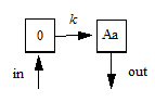
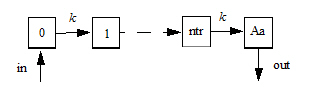
Model for ntr=0 (the smallest possible value)
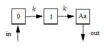
Model for ntr=1
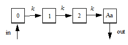
Model for ntr=2
Model for ntr=more
The following model is implemented with extra upstream compartments, and ntr effectively chooses which upstream compartment will be considered compartment 0 and will receive doses:
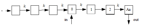
Doses go into compartment 0, as well as any additional rate given by the in keyword. The value is read from the final compartment, which can have a supplemental output rate given by the out keyword. (If artificial dosing is done, such as by saving Aa=Aa+d in a sequence statement, it is understood as adding d to compartment 0, not to compartment Aa.)
The following model shows how the interpolation is done, where x is an auxiliary compartment.
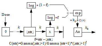
Disclaimer: In the case where ntr is an integer, the transit statement is completely accurate for all inputs. If ntr is not an integer, but dosing consists of bolus doses sufficiently separated in time, it is also completely accurate. However, if ntr is a small non-integer, like 0.5, and multiple boluses occur close together or an infusion is given, the output in Aa is under-predicted by as much as 5%. The under-prediction becomes progressively smaller as ntr increases, but is always zero if ntr is an integer. This is an artifact of the interpolation formula used for fractional values of ntr.
