Graphically create a peripheral elimination model
This example shows how to turn a standard two-compartment model into a model with non-standard elimination by using the graphical editor.
Note:The completed project (Periph_Elim.phxproj) is available for reference in …\Examples\NLME.
Set up the Phoenix Model object
-
Create a new project called Periph Elim.
-
Import the dataset …\Examples\NLME\Supporting files\peripheral elim.dat.
-
Click Finish in the File Import Wizard dialog.
-
Right-click the worksheet and select Send To > Phoenix Modeling > Phoenix Model.
-
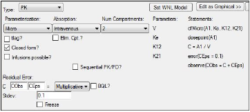
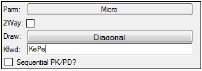
In the Structure tab of the Phoenix model, select Micro from the Parameterization menu.
-
In the Num Compartments menu, select 2.
-
Change C (continuous observation) to a multiplicative error model by selecting Multiplicative in the C error menu.
-
The Stdev field should read 0.1.
Map the model variables
-
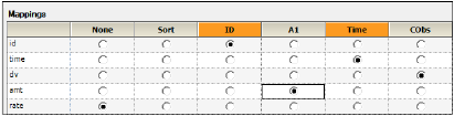
Select the option buttons in the Main Mappings panel to map the data types as follows:
id to the ID context.
time to the Time context.
dv to the CObs context.
amt to the A1 context.
Leave rate mapped to None.
Edit the graphical model
-
Click Edit as Graphical.
-
In the confirmation dialog, click Yes.
-
In a second confirmation dialog about not using the closed-form, click Yes.
-
If needed, click Model in the Phoenix Model object Setup tab list to display the Model diagram panel.
-
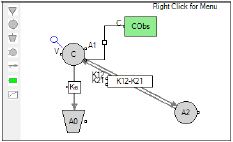
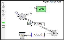
Delete the PK flow between the Central compartment C and the Elimination compartment A0 by selecting the square labeled Ke, then right-clicking and selecting Delete.
-
Confirm the deletion by clicking Yes in the dialog.
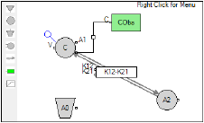
The graphical model now looks like this: -
Add a PK flow between the Peripheral compartment A2 and the Elimination compartment A0.
A PK flow can be added in one of two ways:
Click in the Phoenix Model object toolbox.
Or
Right-click anywhere in the Model diagram panel and select Insert > Flow.
When the PK flow is inserted, the first and second compartments of the flow must be selected.
Left-click the first compartment of the flow, the Peripheral compartment A2.
Left-click the second compartment of the flow, the Elimination compartment A0.
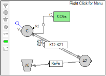
The PK flow is inserted between the two-compartments. -
Select the PK flow named K_A2_A0, if it is not already selected, and type KePe in the Structure tab field Kfwd.
KePe stands for the rate of elimination between the peripheral compartment and the elimination compartment. -
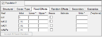
Select the Parameters > Fixed Effects sub-tab.
-
In the Initial column, type the following initial estimates for each of the parameters:
-
Select the Run Options tab.
-
In the Algorithm menu select Naive pooled.
-
Click
 to execute the object.
The first model execution is used to find better initial estimates for the fixed effects. -
Select the Parameters > Fixed Effects sub-tab.
-
Click Accept All Fixed+Random to copy the new estimates to the Initial estimates field for each parameter.
-
Select the Run Options tab.
-
In the Algorithm menu select FOCE L-B.
-
Click
 to execute the object.
|
Parameter |
Initial Value |
|
tvV |
1 |
|
tvK12 |
.01 |
|
tvK21 |
.01 |
|
tvKePe |
.01 |
Save and close the project
-
Select File > Save Project.
-
Click Save.
-
Select File > Close Project.
The project is saved and closed and Phoenix can be safely exited.
This concludes the peripheral elimination model example.
