Fitting PK and PD data and using a simulation run

This example demonstrates a simultaneous fitting of PK and PD data. The PK data follows a one-compartment model with first-order absorption and elimination through oral administration. The PD data can be described using a simple Emax model. Both PK and PD models are found in the Phoenix library models as PK model 3 and PD model 102.

This example also demonstrates the use of the Monte Carlo population simulation that is available when users select the Predictive Check run mode option. Simulation runs can be used when model­ers have PK/PD parameter estimates from prior modeling runs and want to explore the effects of modifying certain conditions, such as dosing regimens, without having to import or create more data.

Note:The completed project (PKPD_Linked.phxproj) is available for reference in …\Exam­ples\NLME.

Set up the Phoenix Model object

1. Create a new project called PKPD Linked.

2. Import the dataset …\Examples\NLME\Supporting files\pkpd.dat.

3. Click Finish in the File Import Wizard dialog.

Filter the effect data

The dataset contains drug concentration and effect data. In order to use the dataset with a linked PK/PD model, the concentration and effect data must be filtered into separate columns, and a column for dosing data must be appended to the final worksheet.

1. Right-click Workflow in the Object Browser and select New > Data > Data Wizard. The Setup tab is displayed in the right viewing panel.

2. Rename the Data Wizard object Filter Effect Data.

3. From the Action menu in the Options tab, select Filter.

4. Click Add.
   The Options tab is populated with tools for defining the filtering criteria to use. The Mappings panel becomes available in the Setup tab and Step 1-No Action is changed to Step 1-Filter in the Setup tab list.

5. Use the mouse pointer to drag the pkpd worksheet from the Data folder to the Main Mappings panel.

6. Use the Specify Filter area of the Options tab to specify a filter for the worksheet. The Built In filter option button is selected by default.

7. Click Add to the left of the Built In option.

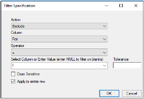
8. In the Filter Specification dialog, leave Exclude selected in the Action menu.

9. In the Column menu select Fcn.

10. In the Select Column or Enter Value field type 1.

11. Leave the Apply to entire row checkbox.

 

12. Click OK.

13. Click to execute the object.

Filter the concentration data

1. Insert a second Data Wizard object into the project.

2. Rename the Data Wizard object Filter Conc Data.

3. From the Action menu in the Options tab, select Filter.

4. Click Add.

5. Use the mouse pointer to drag the pkpd worksheet from the Data folder to the Mappings panel.

6. Use the Options tab to specify a filter for the worksheet. The Built In filter option button is selected by default.

7. Click Add to the left of the Built In option.

8. In the Action menu leave Exclude selected.

9. In the Column menu select Fcn.

10. In the Value field type 2.

11. Leave the Apply to entire row checkbox.

12. Click OK.

13. Click to execute the object.

Merge and transform the filtered worksheets

1. Select the workflow in the Object Browser and then select Insert > Data > Merge Worksheets.

2. In the Worksheet 1 Mappings panel click  to open the Select Source dialog.

3. Select the Filter Effect Data Result worksheet and click OK.

4. Select the option buttons in the Worksheet 1 Mappings panel to map the data types to the follow­ing contexts:
   ID to the Sort context.
   Time to the Sort context.
   Leave Fcn mapped to None.
   DV to the Included Column context.

5. In the Worksheet 2 Mappings panel click  to open the Select Source dialog.

6. Select the Filter Conc Data Result worksheet and click OK.

7. Select the option buttons in the Worksheet 2 Mappings panel to map the data types to the follow­ing contexts:
   ID to the Sort context.
   Time to the Sort context.
   Leave Fcn mapped to None.
   DV to the Included Column context.

8. Click to execute the object.

Add a dosing data column

1. Select the workflow in the Object Browser and then select Insert > Data > Data Wizard.

2. Rename the Data Wizard object Column Transform.

3. From the Action menu in the Options tab, select Transformation.

4. Click Add.
   The Options tab is populated with tools for defining the transformation to take place. The Mappings panel becomes available in the Setup tab and Step 1-No Action is changed to Step 1-Transforma­tion in the Setup tab list.

5. In the Column Transform Main Mappings panel click  to open the Select Source dialog.

6. Select the Merge Worksheets Result worksheet and click OK.

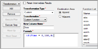
7. In the Options tab, select Custom from the Transformation Type menu.

8. In the New Column Name field, type Dose.

9. In the Formula field, type if(Time=0,100,0).

 

10. In the Main Mappings panel, make sure that Time is mapped to the Time context. Leave all other data types mapped to None.

11. Click to execute the object.

12. Right-click the Result worksheet in the Results tab list and select Copy to Data Folder.

The worksheet is copied to the Data folder and renamed “Result from Column Transform”.

Modify the transformed dataset

1. In the Data folder, rename the “Result from Column Transform” worksheet as PKPD Data.

2. In the Columns tab, located below the right viewing panel, select the DV column header in the Col­umns list.

3. Click DV again to make it editable and type Effect.

4. In the same way, rename the DV_1 column header Conc.

Set up the linked model

The Phoenix Model interface allows users to select compiled WinNonlin PK, PD, or linked PK/PD library models.

1. Select the PKPD Data worksheet in the Data Folder.

2. Right-click the worksheet and select Send To > Phoenix Modeling > Phoenix Model.

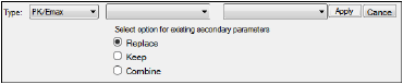
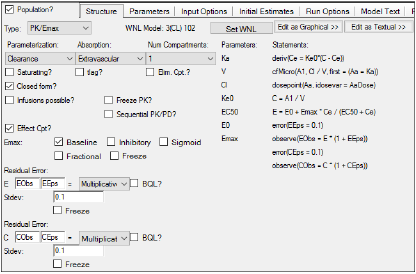
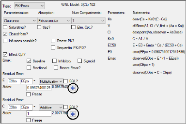
3. In the Structure tab, select PK/Emax in the Type menu.

4. Click Set WNL Model.
   There are two unlabeled menus. The first allows users to select a PK model, and the second allows users to select a PD model.

 

5. In the PK menu (the first unlabeled menu) select Model 3 (3 1cp extravascular).

6. Check the Cl/V checkbox.

7. In the PD menu (the second unlabeled menu) select Model 102 (102 emax base).

8. Click Apply. The WinNonlin model is set.

9. Clear the Freeze PK? checkbox to add a continuous observation to the model.

10. In the E error menu, select Multiplicative.

11. In the C error menu, select Multiplicative.

 

12. Select the Parameters > Structural sub-tab.

13. Clear the Ran checkboxes for Ka and E0.

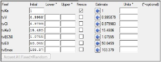
14. Select the Fixed Effects sub-tab.

15. Check the box for tvKa to “freeze” the value.

16. Some of the initial estimates must be changed in order for the model to run correctly.
    In the Initial field for tvKe0, type 10.
    In the Initial field for tvE0, type 50.
    In the Initial field for tvEmax, type 100.

17. Select the Random Effects sub-tab.

18. Type 0.1 in the Initial Estimates fields for nEC50, nEmax, nKe0, nV, and nCl.

19. Select the Run Options tab.

20. In the Algorithm menu, select FOCE L-B.

Map the model variables

1. Select the option buttons in the Main Mappings panel to map the data types as follows:
   ID to the ID context.
   Time to the Time context.
   Effect to the EObs context.
   Conc to the CObs context.
   Dose to the Aa context.

2. Click to execute the object.

Simulate a population model

This part of the example uses the previously created model to run a simulated model by using the Predictive Check run mode option to perform a Monte Carlo population PK/PD simulation.

1. In the Object Browser, right-click the Model object and select Copy.

2. Right-click the Workflow object and select Paste.

3. Rename the project as PKPD Simulation.

4. In the Structure tab, click  beside the effect observation Stdev field to use the new value as the standard deviation.

5. Click  beside the concentration observation Stdev field to use the new value as the standard deviation.

 

6. Select the Parameters > Fixed Effects sub-tab.

7. Click Accept All Fixed+Random to copy the model estimates to the Initial estimate field for each fixed effect parameter.

 

The values entered in the Fixed Effects sub-tab are used for all subjects. Because the input data­set contains multiple subjects, the parameter values are needed to create variations in the simu­lated data.

8. Select the Run Options tab.

9. Select the Simulation run mode.

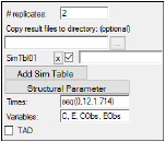
10. In the Simulation Options area, click Add Sim Table to add a simulation table.

11. In the Times field, enter seq(0,12,1.714). This specifies a sequence of times from zero to 12 incremented by 1.714 time units (0, 1.714, 3.428, 5.142, …, 12).

12. In the Variables field, enter C, E, CObs, EObs.
    
    C and E are simulated individual predicted values (simulated IPREDs), and CObs and EObs are simulated observations.

 

13. Click to execute the object.

Simulation output

A simulation worksheet and an external file are created. All other results listed in the Results tab cor­respond to the model fit because Phoenix fits the model before performing simulations.

•PredCheckAll: worksheet containing the predictive check simulated data points.

•Rawsimtbl01.csv: the simulated data. This file is created externally because, depending on the number of replicates, it can be very large and affect performance. This file can be exported or opened in Microsoft Excel.

Save and close the project

1. Select File > Save Project.

2. Click Save.

3. Select File > Close Project.

The project is saved and closed and Phoenix can be safely closed.

This concludes the fitting example.

 

---

Last modified date:6/26/19

Legal Notice | Contact Certara
© 2019 Certara USA, Inc. All rights reserved.