Phoenix PML supports a majority of the intrinsic math functions in the Cmath.h library (see “Supported Math Functions” for a list of supported math functions). In general, the function names are the same or very similar to the Fortran (and hence NONMEM) names of the same functions. There are some differences, however. For example, fabs(x), which applies to floating-point values, computes the absolute value of x. Do not use ABS(x), the Fortran name for absolute value, as this will give incorrect results when called with real number arguments.
In addition to the Cmath.h library functions, Phoenix PML also supports a variety of special functions that are useful in PK/PD modeling, such as the cumulative normal distribution phi(x), the inverse cumulative normal distribution probit(x), the Lambert W-function lambertw(x) for closed-form solutions to one-compartment Michaelis-Menten nonlinear elimination models, as well as various link and inverse link functions, and some special functions useful for defining log likelihoods in certain count-type models. A complete list of special functions is provided in “Supported Special Functions”.
Function names are typically written in lower case. For example, functions like exp, sqrt, log, are lower case, because PML uses the standard C library, in which lower case is the norm. This differs from other programs like NONMEM, which are not case sensitive. Spelling a function name incorrectly will result in a linker error message saying the function is undefined.
If numeric constants are needed in the code, and there is a concern about possible performance of calculating them, a simple way to include them is the following:
double(pi, e)
sequence {
pi=3.1415926535897932384626433832795
e=2.7182818284590452353602874713527
}
These are executed only once per subject, take essentially zero time to execute, and are far more precise than can possibly be required.
Do not be concerned about the performance of secondary parameter calculations, such as half-life, because those are only calculated once, after all model fitting is completed.
Dosing can be specified in two places, the model file and the column definition file. For more, see “Modeling Project Files”.
In the model, the dosepoint statement can contain several options, including:
•tlag=expr dose delivery is delayed by expr
•duration=expr 0-order infusion spanning expr time units
•rate=expr 0-order infusion of expr units/time unit
•bioavail=expr expr is the fraction delivered
The dosepoint statement can also include statements to be executed before and/or after delivery of the dose, as follows.
dobefore=block
doafter=block
Covariates can be simple or interpolated. See “Modeling Project Files” for more information.
covariate(covariate_name)
This specifies that there is a covariate with the given name. For time-varying covariates, the covariate statement extrapolates backward. So, for example, if a covariate is given at time=1, 2, and 3 to be 10, 20, and 30, respectively, then the covariate value in [0,1] is 10, in [1,2] is 20, and in [2,3] is 30.
fcovariate(covariate_name)
This is the same as covariate, except that it also specifies the covariate has forward direction. fcovariate extrapolates forward. So, for example, if a covariate is given at time=1, 2, and 3 to be 10, 20, and 30, respectively, the fcovariate value for [1,2] is 10, for [2,3] is 20, and for times beyond 3 (if any) it is 30. If no covariate value is given at time=0, the fcovariate value for [0,1] is also 10, as the first value propagates backward as well as forward.
There are actually two different ways to indicate forward direction, by using the fcovariate statement in the model text, or by using fcovr in the column definition text (or both).
interpolate(covariate_name)
This also specifies that there is a covariate with the given name, however, the value of the covariate varies linearly between time points at which it is set in time-based models. This feature should be used with caution, because in some cases it makes a linear model nonlinear so it cannot use the matrix exponent ODE solver.
This can happen in a simple PK model parameterized by Cl and V, if V is a function of bodyweight BW, and BW is interpolated. Alternatively if the model is parameterized by Ke and V, it is not affected because V does not enter the differential equations.
covariate(Form())
In a text model, if a covariate is categorical, its name must be followed by empty parentheses. This informs the UI that the covariate is categorical, and thus available for stratification.
There are many kinds of models involving discrete time-based events at which discontinuous changes can occur in a model. The following is a partial example of an entero-hepatic reflux model.
1 deriv(a=-a*k10-a*k1b+g*kg1)
# central cpt
2 deriv(b=a*k1b-qbg)
# bile cpt
3 deriv(g=qbg-g*kg1)
# gut cpt
4 real(qbg)
#qbg is flow rate from bile to gut
5 stparm(tCycle=…, tReflux=…)
# times are parameters
# introduce the time sequence:
6 real(i)
7 sequence{
8 i=0;
9 while(i<10){
10 i=i+1;
11 qbg=0;
12 sleep(tCycle-tReflux);
13 qbg=(b/tReflux);
14 sleep(tReflux);
15 qbg=0;
16 }
17 }
The model has three compartments: a for plasma, b for bile, and g for gut. Normally the compound flows from gut to plasma and from plasma to bile, as well as flowing through the normal elimination path. There is also a flow from bile to gut, which is the reflux path. This is modeled as a zero-order flow of rate qbg. The flow is turned on and off to model the reflux.
Lines 1–3 give the differential equations for the three compartments. The variable qbg is a variable representing the flow rate from bile to gut, and it is initially zero.
Line 4 declares a variable, qbg, which will be used in some of the equations and statements.
Line 5 designates that there are two structural parameters giving the cycle time between reflux events (tCycle) and the duration (tReflux) of each event.
Line 6 declares a variable, i, which will be used in some of the equations and statements.
Lines 7–17 are grouped with the sequence keyword. This introduces time-sequenced procedure into the model.
Line 8 sets the initial value for the variable i to zero.
Line 9 groups the next six statements into a loop that will repeat up to 10 times.
Line 10 adds one to the value of i (number of iterations).
Line 11 sets the initial value for the variable qbg to zero.
Line 12 allows tCycle-tReflux time units to pass.
Line 13 turns on the reflux by setting qbg to the rate necessary to empty the bile compartment within duration tReflux.
Lines 14–15 say to wait for tReflux time units, and then turn off the flow, after which the cycle repeats.
Discrete and distributed delays
Transit compartment models, described by systems of ordinary differential equations (ODEs), have been widely used to describe delayed outcomes in pharmacokinetics and pharmacodynamics studies. The obvious disadvantage for this type of model is it requires manually finding proper values for the number of compartments, and hence it is time-consuming. It is also difficult, if not impossible, to do population analysis using this model. In addition, it may require many differential equations to fit the data and may not adequately describe some complex features.
To alleviate these advantages, a distributed delay approach was proposed in “Hu, Dunlavey, Guzy, and Teuscher (2018)” to model delayed outcomes in pharmacokinetics and pharmacodynamics studies. It involves convolution of the signal to be delayed (S) and the probability density function (g) of the delay time,
|
|
(1) |
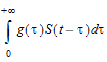
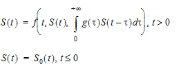
Thus, for the distributed delay approach, the delay time may vary among signal mediators (e.g., drug molecules or cells), and hence it is a natural extension of the discrete delay approach that
|
|
(2) |

in which case, where the delay time is assumed to be the same (i.e., t) for all signal mediators.
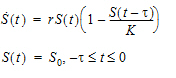
Differential equations involving discrete delays and/or distributed delays are called delay differential equations (DDEs). The difference between ODEs and DDEs is that the future state of the system governed by ODEs is totally determined by its present value while for DDEs it is determined not only by its present value, but also by its past. This means that, for DDEs, one has to specify the values of the system state prior to the system starts (assuming throughout that the system starts at time zero). For example, for the following differential equation with a distributed delay,
|
|
(3) |
one has to specify the values of S(t) over all negative t; that is, one has to specify S0, which is often called the history function.
It was shown in “Hu, Dunlavey, Guzy, and Teuscher (2018)” that the distributed delay approach is general enough to incorporate a wide array of pharmacokinetic and pharmacodynamic models as special cases, including transit compartment models, effect compartment models, indirect response models with production either simulated or inhibited, typical absorption models (either zero-order or first-order absorption), and a number of atypical (or irregular) absorption models (e.g., parallel first-order, mixed first-order, and zero-order, inverse Gaussian, and Weibull absorption models). This was done through assuming a specific distribution form for the delay time.
Specifically, transit compartment models are based on the assumption that the delay time is Erlang distributed, with shape and rate parameters respectively determining the number of transit compartments and the transition rate between the compartments. Note that Erlang distribution is a special case of the gamma distribution, which allows for non-integer shape parameters. Hence, distributed delay models with delay time assumed to be gamma distributed (referred to as gamma distributed delay models) are natural extension of transit compartment models. Examples for extending transit compartment models to their corresponding gamma distributed delay models can be found in “Hu, Dunlavey, Guzy, and Teuscher (2018)” and “Krzyzanski, Hu, and Dunlavey (2018)”.
The delay function in PML can be used for both discrete and gamma distributed delays, and its syntax is given as follows:
delay(S, MeanDelayTime
[, shape=ShapeParam]
[, hist=HistExpression]
)
If the shape option is not provided, then it returns the value of S(t − MeanDelayTime). Otherwise, it returns the value of “1” with g assumed to be the probability density function of a gamma distribution with shape parameter being ShapeParam specified by the shape and mean being MeanDelayTime. The hist option is used to specify the value of S prior to time 0; that is, if t < 0, then S(t)=HistExpression, which is required to be independent of time t, but can depend on variables that are defined at time 0 for the subject, such as covariates, fixed and random effects. If the hist option is not provided, then it is assumed that S(t)=0 for t < 0.
It should be noted that the delay function relies on the fact that ODE solvers use shorter step sizes in the vicinity of rapid changes. Hence, it will not work in the presence of methods that have large step sizes, such as matrix exponent or closed-form. Even though there is no restriction on the number of delay functions put in a model, it should be used sparingly to avoid performance issue.
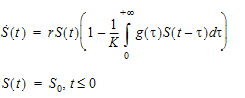
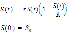
For the discrete delay function, the delay time can be estimated, and for the distributed delay case, both the mean and shape parameter for the gamma distribution can be estimated. In addition, the delay function can be put on the right-hand side of a differential equation, and hence can be used to numerically solve a differential equation with either discrete delays or gamma distributed delays, no matter whether the signal to be delayed, S, depends on model states or not. For example, the delay function can be used to numerically solve the well-known Hutchinson equation (a logistic growth model with a discrete delay):
|
|
(4) |
where r denotes the intrinsic growth rate, K is the carrying capacity, and S0 is a positive constant. The PML code for this model is given as follows:
deriv(S=r*S*(1-delay(S, tau, hist=S0)/K))
sequence{S=S0}
The delay function can also be used to numerically solve the following logistic growth model with a distributed delay:
where g is the probability distribution function of a gamma distribution with shape parameter being ShapeParam and mean being MeanDelayTime. The PML code for this model is given as follows:
delayedS=delay(S, MeanDelayTime,
shape=ShapeParam,
hist=S0
)
deriv(S=r*S*(1-delayedS/K))
sequence{S=S0}
A simple simulation of the logistic growth model with a gamma distributed delay, equation (5), is given in example project LogisticGrowthModelWithGammaDistributedDelay.phxproj (located in …\Examples\NLME). The project demonstrates that equation (5) can exhibit much richer dynamics than its corresponding ODE.
|
|
(6) |
For example, it may produce an oscillation around the carrying capacity while the corresponding ODE cannot. In addition, adjusting the mean delay time can achieve the desired type of oscillations (either damped or sustained oscillations).
Note that, the signal to be delayed, S, in the delay function cannot contain dosing information from the input data set. Hence, it cannot be used for the absorption delay case. To achieve this, a compartment modeling statement, delayInfCpt, was added to PML with its syntax given as follows:
delayInfCpt(A, MeanDelayTime,
ShapeParamMinusOne
[, in=inflow]
[, out=outflow
)
where A denotes a compartment that can receive doses (from the input data set) through the dosepoint statement. Mathematically, this statement means:
|
|
(7) |
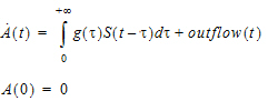
Here S denotes all the input to be delayed, including the dose and the inflow specified by the in option, with S(t)=0 if t < 0, and g is the probability distribution function of a gamma distribution with mean given by MeanDelayTime and shape parameter ν given by:
|
|
(8) |

where ShapeParamMinusOne must be non-negative and is to prevent the shape parameter going from less than one (which cause singularity of g at time 0). The outflow defined by the out option is used to specify additional flow rates (either out of or into compartment A) that are not delayed.
There are two examples that demonstrate how to use delayInfCpt to model absorption delay. For the first one, the delay time between the administration time of the drug and the time when the drug molecules reach the central compartment is assumed to be gamma distributed with the mean given by MeanDelayTime and shape parameter ν given by ν=ShapeParamMinusOne+1. In addition, the drug is assumed to be described by a one-compartment model with a first-order clearance rate. The PML code for the structure model of this example is then given by:
# central compartment
delayInfCpt(A1, MeanDelayTime,
ShapeParamMinusOne,
out =-Cl*C
)
dosepoint(A1)
# drug concentration at the central compartment
C=A1/V
The second example is about double sites of absorption, where the drug is assumed to be described by a two-compartment model with a first-order elimination from the central compartment. In addition, the delay time between the administration time of the drug and the time when the drug molecules reach the central compartment is assumed to be gamma distributed for each pathway. The PML code for the structure model of this example is then given by:
# 1st pathway contribution to the central compartment,
# where frac denotes the fraction of dose absorbed by
# the 1st pathway, and the remaining dose is
# absorbed by the 2nd pathway.
delayInfCpt(Ac1, MeanDelayTime1, ShapeParamMinusOne1,
out=-Cl*C-Cl2*(C-C2)
)
dosepoint(Ac1, bioavail=frac)
# 2nd pathway contribution to the central compartment
delayInfCpt(Ac2, MeanDelayTime2, ShapeParamMinusOne2)
dosepoint(Ac2, bioavail=1-frac)
# Peripheral compartment
deriv(A2=Cl2*(C-C2))
# Drug concentration at the central compartment
C=(Ac1+Ac2)/V
# Drug concentration at the peripheral compartment
C2=A2/V2
The model fitting and visual predictive checks for the first example are demonstrated in the example project ModelAbsorptionDelay_delayInfCpt.phxproj (located in …\Examples\NLME). The project results show that the shape parameter can be reliably estimated along with the other parameters. In addition, standard diagnostic plots and visual predictive checks are good.
Hu, Dunlavey, Guzy, and Teuscher (2018)
A distributed delay approach for modeling delayed outcomes in pharmacokinetics and pharmacodynamics studies. J Pharmacokinet Pharmacodyn. https://doi.org/10.1007/s10928-018-9570-4.
Krzyzanski, Hu, and Dunlavey (2018)
Evaluation of performance of distributed delay model for chemotherapy-induced myelosuppression. J Pharmacokinet Pharmacodyn. https://doi.org/10.1007/s10928-018-9575-z.
sequence(block)
Sequential execution is where there is a sequence of statements A, B, C, etc., where A executes first in time, and only after A completes does B get to start, and so on. If control is sequential, then one can have “if” statements and loops, and variables that act like counters. One can say “x=x + 1” and know what it means, because it takes place at a point in time.
By contrast, in a PML model, the statements are not sequential, they are descriptive of the problem. They do not take action at a point in time. Rather they apply “all the time”. So in PML code, outside of sequence blocks (and assignment statements), relative order of statements does not matter.
The sequence statement denotes a series of expressions to evaluate or statements to process at certain times in a time-based model. The incorporation of sequence blocks into PML allows handling of models like entero-hepatic reflux in a general way.
Processing a block of expressions and statements in a sequence statement is started at the initial time in the model, which is usually zero for differential equation models, and continues until the end of the sequence block, or until a sleep statement is encountered.
Initializing state:
In a sequence block, one can say:
sequence {
Aa=some_expression
A1=some_other_expression
}
This sets the two state variables Aa and A1 to initial values, because the sequence block starts executing immediately when the subject begins.
Take some action after some time has passed:
For example, to put in an extra dose at three time units after the subject has begun, and then yet another three time units later, one could say:
sequence {
sleep(3)
Aa=Aa+some_dose_amount
sleep(3)
Aa=Aa+some_dose_amount
}
The sequence block starts when the subject starts, but the first thing it does is hit the sleep(3) statement, which means “wake up again after three time units”.
When the three time units have passed, then it does the next thing, which is to add a dose to Aa. Notice that an integrator variable like Aa can only be modified at particular points in time, so it can only be modified inside a sequence block.
Then it sleeps for three more time units, gives another dose, and does nothing more.
If there is more than one sequence block, they run on parallel tracks and do not depend on the relative order in which the other sequence blocks do things. For example, if two sequence blocks both initialize things, one cannot depend on which one does the initialization first.
Do different things depending on different conditions:
The following sequence statement begins with sleeping for three time units, then checks if the amount in compartment Aa is less than two. If the amount is less than two, then add a dose to compartment Aa. Otherwise, do something else or do nothing, depending on code that would appear after the else line.
sequence {
sleep(3)
if (Aa < 2){
Aa=Aa+some_dose_amount
} else {
}
}
Do things repeatedly:
The following sequence statement says that, as long as t is less than 10, sleep three time units and then add a dose.
sequence {
while(t < 10){
sleep(3)
Aa=Aa+some_dose_amount
}
}
Alternatively, a variable can be declared that can be set to different values. Then a sequence statement can be used to repeat the sleep + dose cycle ten times, as shown below:
real(i)
sequence {
i=1
while(i <= 10){
sleep(3)
Aa=Aa+some_dose_amount
i=i+1
}
}
group(block)
The group statement ensures that the block assignment statements get executed prior to the stparm statements.
There are two levels of a model:
-
The structural level, which has compartments, doses, and observations, and parameters (called structural parameters)
-
The population level, which has typical values of parameters (fixed effects), inter-individual variation (random effects), covariates, and covariate effects (which are also fixed effects)
The statement that ties the two levels together is called stparm. It defines each structural parameter as a function of fixed effects, covariates, and random effects for estimation and simulation.
Sometimes, to simplify the stparm statements, it is desirable to calculate parts of them outside in separate statements. This cannot be done with ordinary assignment statements like A=B+C, but it can be done inside a group statement, like group(A=B+C), where B and C can only be functions of covariates and fixed effects. Then A is called a group parameter and it can be used in the right-hand-side of an stparm statement. In situations with complex covariate effects, this can lead to substantial performance improvement, by avoiding frequent calls to math functions.
Example 1:
A covariate model can be defined in using standard PML, as follows:
stparm(V=((Gender==0) ? tvV: tvV *dVdGender)*exp(nV))
If the user prefers separate lines, each group can be defined separately (by combining covariate values):
group(
tvVMale=tvV
tvVFemale=tvV *dVdGender
stparm(V=((Gender==0) ? tvMale : tvFemale)*exp(nV))
)
Example 2:
The following calculates body surface area (BSA) in a group statement using covariates weight (WT) and height (HT), and is only done when covariates change, not on every ODE evaluation. This group statement avoids the calculation of BSA at each iteration of ODE solver steps.
covariate(WT) # WT: body weight
covariate(HT) # HT: height
# BSA: body surface area
group(BSA=(WT^0.5378)*(HT^0.3964)*0.024265)
sleep(number)
This statement instructs the processing of the statements and expressions in the current sequence block to stop for the amount of time specified by the number argument. The number argument is a relative time, not an absolute time.
The block inside a sequence statement can consist of multiple blocks controlled by logical switches. For instance, in the example above, the expressions and statements inside the sequence statement are contained within a while block which instructs the sequence to repeat itself through the entire time period that observations are made.
It is important to use the sleep statement rather than tests against the time variable to ensure the stability of the algorithms. For example, write {sleep(10); A0=0} and not {if(t=10);A0=0}. The latter does not function as is intended. For a model to work, the sequence statement must be used any time a user would otherwise intend to write something like: if(t>=Tmax){do stuff}.
There can be multiple sequence statements in a model, and they are executed as if they were running in parallel. No assumption should be made about which sequence statement is processed first. When a reset is encountered in the data, due to mapping a reset column, the sequence statement(s) are restarted.
Time event switching in PML versus WinNonlin ASCII models
The while or if statements that were required to switch between time events in the WinNonlin ASCII model do not work as effectively as the sleep statement in the PML. Using the sequence statement in conjunction with the sleep statement is the best way to switch between time events in Phoenix text models.
If a user uses if statements to perform these tasks in the PML, the integrator can jump over the time point of interest. The Jacobian matrix it computes will be very inaccurate because the derivatives are different on each side of the discontinuity. The integrator goes back and forth trying to reduce the compounding errors that it sees, which can cause the integrator to miss the time point of interest.
The stability that the sequence statement offers allows models to be solved more quickly and accurately.
What the sequence statement with sleep statements does is stop the integrator at the appropriate times to make state changes, like RESET or DOSING, or set time discontinuous variables.
The fixef statement declares zero or more fixed effect parameters. There can be more than one such statement in a model.
1 fixef(a
2 b=6.02
3 c(freeze)=3.14
4 d=c(0.01, 0.1, 5)
5 e=c(0.01, 0.1, 5)
6 f(enable=c(1))=c(0.01, 0.1, 5)
7 )
In this example a, b, c, d, e, and f are fixed effect parameters.
Line 1 says that a is a fixed effect parameter.
Line 2 gives b an initial value of 6.02.
Line 3 gives c a fixed, non-estimated initial value.
Line 4 gives d an initial value of 0.1, and provides a lower bound of 0.01 and an upper bound of five.
Line 5 is like line 4.
Note:Any of the lower bounds or upper bounds can be omitted in the above statements.
Line 6 is like line 4, but the fixed effect f is enabled within an estimation run. This is used in covariate effect modeling procedures. Enabling the fixed effect means that it is estimated. If a fixed effect is disabled, that means its value is frozen to 0.0 and it is not estimated. There is a command-line argument, /xe, that determines which variables are chosen to be disabled. If there is no such argument, all fixed effects having an enable clause are disabled.
Rules for using boundaries and initial estimates:
If bounds are used, a log-transformation is used to find the values closest to the boundaries. Boundaries cannot be solved.
Note:It is best practice to try to solve the model without first using boundaries.
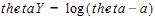
If a one-sided lower bound is used, then the log-transformation is:
If a one-sided upper bound is used, then the log-transformation is:
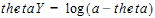
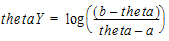
In the above equations, thetaY is the unconstrained transformed variable, and a < theta.
However, if a < theta <b, then:
Fixed effect initial values must be a numerical value. Functions, such as log or exponent, cannot be used as initial estimates. The PML wants a numerical value, not a function. This is similar to how NONMEM works.
Correct: Fixef tvV=C(, 0.7,)
Incorrect: Fixef=tvV=C(, log(C),)
Random effect parameter syntax
The ranef statement specifies zero or more random effect parameters and their covariance structure.
1 ranef(eta1
2 eta2=6
3 diag(eta3, eta4)
4 diag(eta5, eta6)=c(2, 3,)
5 same(eta7, eta8)
6 block(eta9, eta10)
7 block(eta11, eta12)=c(1, 2, 3)
8 block(eta13, eta14)(freeze)=c(1, 2, 3)
9 )
Line 1 says eta1 is a random effect parameter that has its own variance independent of the others parameters. No upper or lower bounds are used, and the initial estimate of variance is one, the default.
Line 2 says eta2 is independent and that the initial estimate of its variance is six. When no initial estimate of variance value is given, the PML uses a default value of one.
Line 3 says eta3 and eta4 have a diagonal variance-covariance matrix. The initial estimate of variance is one, the default.
Line 4 is like line 3, and the function c of the diagonal variance-covariance matrix is given.
Line 5 says that eta7 and eta8 have the same diagonal variance-covariance matrix initial estimate as line 4. Also, the covariance matrix is constrained to be the same as in the previous block. The random effects are different, but drawn from the same distribution as those specified on line 4.
Line 6 says that eta9 and eta10 have a full variance-covariance matrix. The initial estimate of variance for both parameters is one, the default.
Line 7 is like line 6 and gives an initial estimate of the lower triangle of the matrix in row-wise order.
Line 8 is like line 7 and says that the matrix is fixed and is not estimated.
