Phoenix can compute summary statistics for variables in any worksheet. This feature is frequently used to create data to plot means and standard errors, for preclinical summaries, to summarize modeling results, or to test for normal distribution of data. Separate statistics for subgroups are obtained through the use of one or more sort variables.
Use one of the following to add a Descriptive Statistics object to a Workflow:
Right-click menu for a Workflow object: New > NCA and Toolbox > Descriptive Stats.
Or Main menu: Insert > NCA and Toolbox > Descriptive Stats.
Or right-click menu for a worksheet: Send To > NCA and Toolbox > Descriptive Stats.
Note:To view the object in its own window, select it in the Object Browser and double-click it or press ENTER. All instructions for setting up and execution are the same whether the object is viewed in its own window or in Phoenix view.
This section includes information on the following:
•Statistical results and computational formulas
Use the Main Mappings panel to identify which variables are used to compute statistics or weight the data. Required input is highlighted orange in the interface.
None: Data types mapped to this context are not included in any computation or output.
Summary: The variable(s) for which statistics are computed.
Sort: Categorical variable(s) identifying individual data profiles, such as subject ID or gender. Separate statistics are computed for each unique combination of sort variables.
Weight: If a weight variable is present in the dataset, it can be used to weight the summary statistics. If a weight is non-numeric or missing, the observation is excluded from the analysis. If a weight is negative, it is changed to zero (0) upon execution.
See “Statistical results and computational formulas” for a full list of the available statistics.
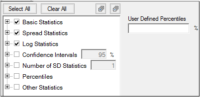
Use the tree on the right to select the statistics to compute and include in the report by checking the corresponding checkboxes.
The available statistics are grouped into categories and checking/unchecking a category checkbox controls all of the checkboxes for statistics within that category. For example, unchecking the Spread Statistics checkbox unchecks the Min, Median, Max, and Range checkboxes.
Click the Select All or Clear All buttons to quickly check/uncheck all checkboxes in the list, respectively, with a single click.
Click the  button to expand all categories in the tree. Click the
  button to collapse all categories in the tree.
There are a number of preset percentiles available in the Percentiles category (1, 2.5, 5, 10, 25, 50, 75, 90, 95, 97.5, 99). However, if you wish to include other percentiles, enter them as a comma-separated list in the User-specified percentiles field.
To generate confidence interval statistics, type the desired confidence interval in the Confidence Interval field.
Check the Confidence Intervals checkbox to compute all statistics in that category or expand the category to select a subset of the statistics
To generate standard deviation statistics, type the desired number of standard deviations in the Number of SD Statistics field. The value must be greater than 0 and less than or equal to 10.
Check the Number of SD Statistics checkbox to compute all statistics in that category or expand the category to select a subset of the statistics.
Statistical results and computational formulas
The Descriptive Stats object creates a Statistics worksheet and a Settings text file in the Results tab. The Statistics worksheet includes summaries of all statistical computations. The Settings file contains user-specified settings.
This table lists all possible descriptive statistics output.
|
Statistic |
Description |
|
CI GEO X% Lower |
Lower limit of an X% confidence interval for the logs of the data, back-transformed to original scale: |
|
CI GEO X% Upper |
Upper limit of an X% confidence interval for the logs of the data, back-transformed to original scale: |
|
CI X% Lower |
Lower limit of an X% confidence interval for the data (i.e., confidence interval that tells the range that is expected to have X% of the data): |
|
CI X% Lower GEO Mean |
Lower limit of an X% confidence interval for the Geometric Mean: |
|
CI X% Lower Mean |
Lower limit of an X% confidence interval for the mean (i.e., the confidence interval in which the mean exists with X% certainty): |
|
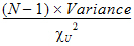
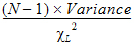
CI X% Lower Var |
Lower limit of an X% confidence interval for the variance (i.e., the confidence interval in which the variance exists with X% certainty): |
|
CI X% Upper |
Upper limit of an X% confidence interval for the data: |
|
CI X% Upper GEO Mean |
Upper limit of an X% confidence interval for the Geometric Mean: |
|
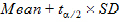
CI X% Upper Mean |
Upper limit of an X% confidence interval for the mean: |
|
CI X% Upper Var |
Upper limit of an X% confidence interval for the variance: |
|
CV% |
Coefficient of variation: (SD/Mean)*100 |
|
GEO Lower XSD and GEO Upper XSD |
Range determined by adding or subtracting “X” log standard deviations from the log-mean, back-transformed to original scale: |
|
Geometric CV% |
Geometric coefficient of variation. |
|
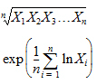
Geometric Mean |
Nth root of the product of the N observations. Equivalently, the exponential of the Mean_Log. Each value must be > zero. |
|
Geometric SD |
Geometric standard deviation of the natural logs of the observations: |
|
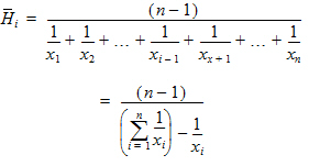
Harmonic Mean |
Reciprocal of the arithmetic mean of the reciprocals of the observations: |
|
IQR |
Interquartile range is the difference between the first and third quartiles (i.e., the middle 50% of the data). IQR is only included in the output when the Include Percentiles checkbox is checked. |
|
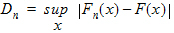
Kolmogorov-Smirnov normality test The Kolmogorov-Smirnov statistic for a given cumulative distribution function F(x) is: |
|
|
Kurtosis |
Sample coefficient of excess (sample excess kurtosis): |
|
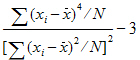
Kurtosis Pop |
Population coefficient of excess (population excess kurtosis): |
|
Lower XSD and Upper XSD |
Range determined by adding or subtracting X standard deviations from the mean: |
|
Max |
Maximum value |
|
Mean |
Arithmetic average |
|
Mean log |
Arithmetic average of the natural logs of the observations: |
|
Median |
Median value — from the percentiles computations, 50th percentile. |
|
Min |
Minimum value |
|
N |
Number of observations with non-missing data (i.e., numeric observations). |
|
Nmiss |
Number of observations with missing data (i.e., non-numeric observations such as text or blanks). |
|
Nobs |
Number of observations (i.e., N+NMiss) |
|
The Pth percentile divides the distribution at a point such that P percent of the distribution are below this point. |
|
|
Pseudo SD |
Jackknife estimate of the standard deviation of the harmonic mean. |
|
Range |
Range of values (maximum value minus minimum value). |
|
SD |
Standard Deviation: |
|
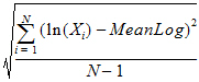
SD Log |
Standard deviation of the natural logs of the observations: |
|
SE |
Standard Error: |
|
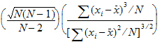
Skewness |
Sample coefficient of skewness (sample skewness): |
|
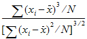
Skewness Pop |
Population coefficient of skewness (population skewness): |
|
Sum |
Sum of the values in the column mapped to Summary. |
|
Variance |
Unbiased sample variance: |
 x
x  x
x  x
x  x
x 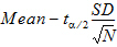


 x
x 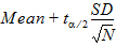


 value. This quantifies the distance between the empirical distribution function of the data and the cumulative distribution function of the Normal distribution.
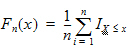
 is the indicator function and
 -value is then computed to determine the significance of
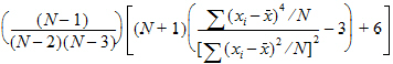


When summary statistics are calculated for a variable with units, some of the output will have units. Assuming that the variable summarized is x and has x-units specified, the units for the summary statistics are:
|
Statistic |
Units |
|
N, Nmiss, Nobs |
No units |
|
CV%, Geometric CV% |
No units |
|
Skewness, Skewness Pop, |
No units |
|
Mean Log, SD Log |
No units |
|
Variance |
x-unit2 |
|
CI Lower Var, CI Upper Var |
x-unit2 |
|
Everything else |
x-unit |
If more than one Summary variable is mapped, with at least two of those variables having units in the input dataset, and the units differ, a stacked Units column is displayed in the Statistics output worksheet that reports the units of the Summary variables. In cases where the input data does not have units, or the units are all the same, then the units of the statistics are displayed in the column headers.
Summary statistics can be weighted by selecting a column in the dataset in the Main Mappings panel to provide weights. If a weight is non-numeric or missing, the observation is excluded from the analysis. Weighted descriptive statistics output also includes a text file called Settings that contains user-specified settings. Some summary statistics and all percentiles are excluded in weighted output.
Results and computational formulas for weighted calculations
The output for weighted summary statistics contains a column indicating the summary variable(s), one for each sort variable, and the statistics listed below.
|
Statistic |
Description |
|
CI X% Lower |
Lower limit of an X% confidence interval for the weighted data: |
|
CI X% Lower Mean |
Lower limit of an X% confidence interval for the weighted mean. |
|
CI X% Lower Var |
Lower limit of an X% confidence interval for the weighted variance. |
|
CI X% Upper |
Upper limit of an X% confidence interval for the weighted data: |
|
CI X% Upper Mean |
Upper limit of an X% confidence interval for the weighted mean. |
|
CI X% Upper Var |
Upper limit of an X% confidence interval for the weighted variance. |
|
CV% |
Weighted coefficient of variation: |
|
Kurtosis Pop |
Weighted coefficient of excess (population excess kurtosis): |
|
Lower XSD and Upper XSD |
Range determined by adding or subtracting X weighted standard deviations from the weighted mean: |
|
Max |
Maximum value |
|
Mean |
Weighted arithmetic average: |
|
Min |
Minimum value |
|
N |
Number of non-missing observations (including those with weights=zero) |
|
Nmiss |
Number of observations with missing data |
|
Nobs |
Number of observations (including observations with weights=zero) |
|
Range |
Range of values (maximum value minus minimum value) |
|
SD |
Weighted standard deviation: |
|
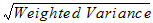
SE |
Weighted standard error: |
|
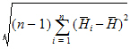
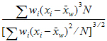
Skewness Pop |
Weighted coefficient of skewness (population skewness): |
|
Sum |
Weighted Sum: |
|
Variance |
Weighted variance: |
 x
x  x
x 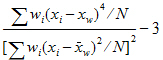


 is the weighted mean.