Use the Main Mappings panel to identify how input variables are used in the Deconvolution object. Deconvolution requires a dataset containing time and concentration data, and sort variables to identify individual profiles. Required input is highlighted orange in the interface.
•None: Data types mapped to this context are not included in any analysis or output.
•Sort: Categorical variable(s) identifying individual data profiles, such as subject ID in a deconvolution analysis. A separate analysis is performed for each unique combination of sort variables.
•Time: The relative or nominal dosing times used in a study.
•Concentration: The measured amount of a drug in blood plasma.
Note:When the column mapped for Time is positioned in the dataset after the column mapped for Concentration, Deconvolution may yield the error message “Time must be sorted in increasing order,” even when the values actually are in increasing order. The workaround is to switch the order of the Time and Concentration columns in the input dataset.
The Deconvolution object assumes a unit impulse response function (UIR) of the form:
|
|
(1) |
where N is the number of exponential terms.
Use the Exponential Terms panel to enter values for the A and alpha parameters. For oral administration, the user should enter values such that:
|
|
(2) |

Required input is highlighted orange in the interface.
•None: Data types mapped to this context are not included in any analysis or output.
•Sort: Categorical variable(s) identifying individual data profiles, such as subject ID.
•Parameter: Data variable(s) to include in the output worksheets.
•Value: A (coefficients) and Alpha (exponential) parameter values.
A and alpha parameters are listed sequentially based on the number of exponential terms selected. If only one exponential term is selected, each profile has an A1 and an Alpha1 parameter. If two exponential terms are selected, each profile has an A1 and an A2 parameter, and an Alpha1 and an Alpha2 parameter.
Rules for using an external exponential terms worksheet:
-
The sort variables must match the sort variables used in the main input dataset.
-
The worksheet’s parameter column must match the number of exponential terms selected in the Exponential Terms menu. For example, if three exponential terms are selected, then each profile in the exponential terms worksheet must have three A parameters and three alpha parameters.
-
The units used for the A and alpha parameters must match the units used for the concentration and dosing data. For example, If the concentration data has units ng/mL and the dosing data has units mg, then the A units must be ng/mL/mg, or the input data or dosing data should be converted (using Data Wizard Properties) to have consistent units. If the time units are hr, then the alpha units are 1/hr.
-
If the UIR parameters are unknown, but a dataset is available that represents the impulse response, the parameters can be estimated by fitting the data in Phoenix with PK model 1, 8, or 18 (for N=1, 2, or 3, respectively). Since the UIR is the response to one dose unit, for model 1 (one-compartment), the inverse of the model parameter V is used for the UIR parameter, i.e., A1=1/V. For model 8 (two-compartment), the model parameters A and B should be divided by the stripping dose to obtain A1 and A2 for the UIR, and similarly for model 18 (three-compartment). However, if the dose units are different than the concentration mass units, the ‘A’ parameters must be adjusted so that the units are in concentration units divided by dose units. For the example in the prior bullet, if A=1/V from model 1 has units 1/mL, then ‘A’ must be converted to ng/mL/mg before it is used for the UIR in the Deconvolution object, A=10^6/V.
Supplying dosing information using the Dose panel is optional. Without it, the Deconvolution object runs correctly by assuming a dose at time zero time-concentration data with the fraction absorbed approaching a final value of one. The dose time is assumed to be zero for all profiles.
Note:The sort variables in the dosing data worksheet must match the sort variables used in the main input dataset.
Required input is highlighted orange in the interface.
•None: Data types mapped to this context are not included in any analysis or output.
•Sort: Categorical variable(s) identifying individual data profiles, such as subject ID.
•Dose: The amount of drug administered.
If the Use times from a worksheet column option button is selected in the Options tab, then the Observed Times panel is displayed in the Setup list. Required input is highlighted orange in the interface.
•None: Data types mapped to this context are not included in any analysis or output.
•Time: Time values.
•Sort: Sort variables.
Note:The observed times worksheet cannot contain more than 1001 time points.
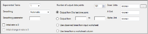
The Options tab allows users to specify settings for exponential terms, parameters, and output time points.
-
In the Exponential Terms menu, select the number of exponential terms in the unit impulse response to use per profile (up to nine exponential terms can be added).
-
In the Smoothing menu, select the method Phoenix uses to determine the dispersion parameter.
•Automatic tells Phoenix to find the optimal value for the dispersion parameter delta.
•None disables smoothing that comes from the dispersion function. If selected, the input function is the piecewise linear precursor function.
•User allows users to type the value of the dispersion parameter delta as the smoothing parameter. The delta value must be greater than zero. Increasing the delta value increases the amount of smoothing.
-
In the Smoothing parameter field, enter the value for the smoothing parameter.
This option is only available if User is selected in the Smoothing menu. -
Select the Initial rate is 0 checkbox to set the estimated input rate to zero at the initial time or lag time.
-
Select the Initial Change in Rate is 0 checkbox to set the derivative of the estimated input rate to zero at the initial time or lag time.
This option is only available if the Initial rate is 0 checkbox is selected. -
In the Dose Units field, type the dosing units to use with the dataset.
•Click the Units Builder  button to use the Units Builder dialog to add dosing units.
•See “Using the Units Builder” for more details on this tool.
-
In the Number of output data points box, type or select the number of output data points to use per profile.
The maximum number of time points allowed is 1001. -
Select the Output from 0 to last time point option button to have Phoenix generate output at even intervals from time zero to the final input time point for each profile.
-
Select the Output from _ to _ option button to have Phoenix generate output at even intervals between user-specified time points for each profile.
•Type the start time point in the first field and type the end time point in the last field.
-
Select the Use observed times from input worksheet option button to have Phoenix generate output at each time point in the input dataset for each profile.
-
Select the Use times from a worksheet column option button to use a separate worksheet to provide in vivo time values.
•Selecting this option creates an extra panel called Observed Times in the Setup tab list.
•Users must map a worksheet containing time values used to generate output data points to the Observed Times panel.
•The observed times worksheet cannot contain more than 1001 time points.
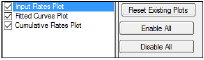
The Plots tab allows users to select whether or not plots are included in the output.
-
Use the checkboxes to toggle the creation of graphs.
-
Click Reset Existing Plots to clear all existing plot output.
Each plot in the Results tab is a single plot object. Every time a model is executed, each object remains the same, but the values used to create the plot are updated. This way, any styles that are applied to the plots are retained no matter how many time the model is executed.
Clicking Reset Existing Plots removes the plot objects from the Results tab, which clears any custom changes made to the plot display. -
Use the Enable All and Disable All buttons to check or clear all checkboxes for all plots in the list. These buttons are most useful when there are many plots listed.
