Options tab

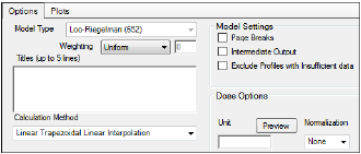
The Options tab allows users to select the WagnerNelson model and set options for the selected model.

 

• Use the Weighting menu to select the regression that estimates Lambda Z or slopes. Available options include:

•User Defined

•Uniform

•1/Y

•1/(Y*Y)

Note:The relative proportions of the weights are important, not the weights themselves. See “Weighting” in the WinNonlin NCA section for more on weighting schemes.

When selecting a weighting model, there are a couple of rules to consider:

If User Defined is selected then users can enter their own Observed to Power N value. The value of N must be typed in the Weighting text field.

When a log-linear fit is done (Uniform weighting for Lambda Z), then the fit is implicitly using a weighting approximately equal to 1/Yhat².

Note:If 1/Y and the Linear Log Trapezoidal calculation method are selected, a user could assume that the weighting scheme is 1/LogY, rather than 1/Y. However, this is not the case because concentra­tions between zero and one would have negative weights, and could not be included in the analy­sis.

• Use the Titles text box to type a title for the analysis.
  
  The title is displayed at the top of each page in the Core output. The title can include up to five lines of text.

• Use the Calculation Method menu to select a calculation method.
  
  Four methods are available for the calculation of area under the curve. The chosen method applies to all AUC and AUMC computations. All methods reduce to the log trapezoidal rule, the linear trapezoidal rule, or both. The methods differ based on when the rules are applied. See “Partial Area Calculation” for descriptive equations of the calculation methods.

•Linear_Log_Trapezoidal: uses the log trapezoidal rule after Cmax, or after C0 if C0 > Cmax. Otherwise the linear trapezoidal rule is used. If Cmax is not unique, then the first maximum is used. This method uses linear trapezoids before Tmax and log trapezoids after Tmax.

•Linear_Trapezoidal_Linear_Interpolation: This is the default method. It applies the linear trapezoidal rule to each pair of consecutive points in the dataset that have non-missing val­ues, and sums up these areas. This method uses linear trapezoids before and after Tmax.

•Linear_Up_Log_Down: uses the linear trapezoidal rule any time that the concentration data is increasing, and the logarithmic trapezoidal rule is used any time that the concentration data is decreasing. This method uses linear trapezoids up and logarithmic trapezoids down before Tmax and linear trapezoids up and logarithmic trapezoids down after Tmax.

•Linear_Trapezoidal_LinearLog_Interpolation: this method is the same as Linear_Trape­zoidal_Linear_Interpolation. It is used when a final time point, that is not in the dataset, is used for predictions. In that case, Phoenix inserts a final concentration value using the Lin­ear_Trapezoidal_Linear_Interpolation rule. If the final time point is after Cmax, or after C0 if C0 > Cmax, the Linear_Trapezoidal_LinearLog_Interpolation rule is used. If Cmax is not unique, then the first maximum is used. This method uses linear trapezoids before and after Tmax.

Note:The Linear Log Trapezoidal, the Linear Up Log Down, and the Linear Trapezoidal Linear/Log Interpolation methods all apply the same exceptions in area calculation and interpolation. If a Y value (concentration, rate, or effect) is less than or equal to zero, Phoenix defaults to the linear trapezoidal or linear interpolation rule for that point. If adjacent Y values are equal to each other, Phoenix defaults to the linear trapezoidal or linear interpolation rule.

No interpolation is performed in the Loo-Riegelman model.

• Select the Page Breaks checkbox to include page breaks in the text output.

• Select the Intermediate Output checkbox to set text output to only include values for iterations during estimation of Lambda Z or slopes, and for each of the sub-areas in partial area computa­tions.

• Select the Exclude Profiles with Insufficient data checkbox to exclude profiles with all or many missing parameter estimates from the results.
  
  If this option is not selected, profiles with insufficient data will have missing output parameter val­ues. See “Data deficiencies resulting in missing values for PK parameters” for a list of cases that produce missing estimates and are excluded by selecting this option.

To set the dosing unit

• Type the dosing unit into the Unit field.

• Click Preview to see a preview of dose option selections.
  The preview is opened in its own window. Click OK to close the preview window.

• Use the Normalization menu to select the appropriate factor if the dose amount is normalized by subject body weight or body mass index. Normalization menu options include:

•None 

•kg 

•g 

•mg 

•m**2 

•1.73 m**2 

If doses are in milligrams per kilogram of body weight, select mg as the dosing unit and kg as the dose normalization. The Normalization menu affects the output parameter units. For example, if dose volume is in liters, selecting kg as the dose normalization changes the units to L/kg. Dose normalization affects units for all volume and clearance parameters, as well as AUCinf/D values.

Plots tab

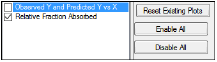
In the Plots tab, users can select whether or not to produce plot output.

 

• Use the checkboxes to toggle the creation of graphs.

• Click Reset Existing Plots to clear all existing plot output.
  
  Each plot in the Results tab is a single plot object. Every time a model is executed, each object remains the same, but the values used to create the plot are updated. This way, any styles that are applied to the plots are retained no matter how many time the model is executed.
  
  Clicking Reset Existing Plots removes the plot objects from the Results tab, which clears any custom changes made to the plot display.

• Use the Enable All and Disable All buttons to check or clear all checkboxes for all plots in the list. These buttons are most useful when there are many plots listed.

Results

 

Users can double-click a plot in the Results tab to edit it. (See the menu options descriptions in the Plots chapter of the Data Tools and Plots Guide for plot editing options.)

 

---

Last modified date:5/30/19

Legal Notice | Contact Certara
© 2019 Certara USA, Inc. All rights reserved.