Deconvolution through convolution methodology
Phoenix deconvolution uses the basic principle of deconvolution through convolution (DTC) to determine the input function. The DTC method is an iterative procedure consisting of three steps. First, the input function is adjusted by changing its parameter values. Second, the new input function is convolved with cd(t) to produce a calculated drug level response. Third, the agreement between the observed data and the calculated drug level data is quantitatively evaluated according to some objective function. The three steps are repeated until the objective function is optimized. DTC methods differ basically in the way the input function is specified and the way the objective function is defined. The objective function may be based solely on weighted or unweighted residual values, or observed–calculated drug levels. The purely residual-based DTC methods ignore any behavior of the calculated drug level response between the observations.
The more modern DTC methods, including Phoenix’s approach, consider both the residuals and other properties such as smoothness of the total fitted curve in the definition of the objective function. The deconvolution method implemented in Phoenix is novel in the way the regularization (smoothing) is implemented. Regularization methods in some other deconvolution methods are done through a penalty function approach that involves a measurement of the smoothness of the predicted drug level curve, such as the integral of squared second derivative.
The Phoenix deconvolution method instead introduces the regularization directly into the input function through a convolution operation with the dispersion function, fd(t). In essence, a convolution operation acts like a “washout of details”, that is a smoothing due to the mixing operation inherent in the convolution operation. Consider, for example, the convolution operation that leads to the drug level response c(t). Due to the stochastic transport principles involved, the drug level at time t is made up of a mixture of drug molecules that started their journey to the sampling site at different times and took different lengths of time to arrive there. Thus, the drug level response at time t depends on a mixture of prior input. It is exactly this mixing in the convolution operation that provides the smoothing. The convolution operation acts essentially as a low pass filter with respect to the filtering of the input information. The finer details, or higher frequencies, are attenuated relative to the more slowly varying components, or low frequency components.
Thus, the convolution of the precursor function with the dispersion function results in an input function, f(t), that is smoother than the precursor function. Phoenix allows the user to control the smoothing through the use of the smoothing parameter d. Decreasing the value of the dispersion function parameter d results in a decreasing degree of smoothing of the input function. Similarly, larger values of d provide more smoothing. As d approaches zero, the dispersion function becomes equal to the so-called Dirac delta “function”, resulting in no change in the precursor function.
The smoothing of the input function, f(t), provided by the dispersion function, fd(t), is carried forward to the drug level response in the subsequent convolution operation with the unit impulse response function (cd). Smoothing and fitting flexibility are inversely related. Too little smoothing (too small a d value) will result in too much fitting flexibility that results in a “fitting to the error in the data.” In the most extreme case, the result is an exact fitting to the data. Conversely, too much smoothing (too large a d value) results in too little flexibility so that the calculated response curve becomes too “stiff” or “stretched out” to follow the underlying true drug level response.
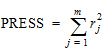
Phoenix's deconvolution function determines the optimal smoothing without actually measuring the degree of smoothing. The degree of smoothing is not quantified but is controlled through the dispersion function to optimize the “consistency” between the data and the estimated drug level curve. Consistency is defined here according to the cross validation principles. Let rj denote the differences between the predicted and observed concentration at the j-th observation time when that observation is excluded from the dataset. The optimal cross validation principle applied is defined as the condition that leads to the minimal predicted residual sum of squares (PRESS) value, where PRESS is defined as:
|
|
(14) |
For a given value of the smoothing parameter d, PRESS is a quadratic function of the wavelet scaling parameters x. Thus, with the non-negativity constraint, the minimization of PRESS for a given d value is a quadratic programming problem. Let PRESS (d) denote such a solution. The optimal smoothing is then determined by finding the value of the smoothing parameter d that minimizes PRESS (d). This is a one variable optimization problem with an embedded quadratic-programming problem.
Phoenix's deconvolution function permits the user to override the automatic smoothing by manual setting of the smoothing parameter. The user may also specify that no smoothing should be performed. In this case the input rate function consists of the precursor function alone.
Besides controlling the degree of smoothing, the user may also influence the initial behavior of the estimated input time course. In particular the user may choose to constrain the initial input rate to zero (f(0)=0) and/or constrain the initial change in the input rate to zero (f'(0)=0). By default Phoenix does not constrain either initial condition. Leaving f(0) unconstrained permits better characterization of formulations with rapid initial “burst release,” that is, extended release dosage forms with an immediate release shell. This is done by optionally introducing a bolus component or “integral boundary condition” for the precursor function so the input function becomes:
|
f(t)=fp(t)*fd(t)+xd fd(t) |
(15) |
where the fp(t)*fd(t) is defined as before.
The difference here is the superposition of the extra term xd fd(t) that represents a particularly smooth component of the input. The magnitude of this component is determined by the scaling parameter xd, which is determined in the same way as the other wavelet scaling parameters previously described.
The estimation procedure is not constrained with respect to the relative magnitude of the two terms of the composite input function given above. Accordingly, the input can “collapse” to the “bolus component” xd fd(t) and thus accommodate the simple first-order input commonly experienced when dealing with drug solutions or rapid release dosage forms. A drug suspension in which a significant fraction of the drug may exist in solution should be well described by the composite input function option given above. The same may be the case for dual release formulations designed to rapidly release a portion of the drug initially and then release the remaining drug in a prolonged fashion. The prolonged release component will probably be more erratic and would be described better by the more flexible wavelet-based component fp(t)*fd(t) of the above dual input function.
Constraining the initial rate of change to zero (f'(0)=0) introduces an initial lag in the increase of the input rate that is more continuous in behavior than the usual abrupt lag time. This constraint is obtained by constraining the initial value of the precursor function to zero (fp(0)=0). When such a constrained precursor is convolved with the dispersion function, the resulting input function has the desired constraint.
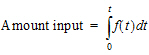
The extent of drug input in the Deconvolution object is presented in two ways. First, the amount of drug input is calculated as:
|
|
(16) |
Second, the extent of drug input is given in terms of fraction input. If test doses are not supplied, the fraction is defined in a non-extrapolated way as the fraction of drug input at time t relative to the amount input at the last sample time, tend:
|
|
(17) |
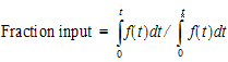
The above fraction input will by definition have a value of one at the last observation time, tend. This value should not be confused with the fraction input relative to either the dose or the total amount absorbed from a reference dosage form. If dosing data is entered by the user, the fraction input is relative to the dose amount (i.e., dose input on the dosing sheet).
Charter and Gull (1987). J Pharmacokinet Biopharm 15, 645–55.
Cutler (1978). Numerical deconvolution by least squares: use of prescribed input functions. J Pharmacokinet Biopharm 6(3):227–41.
Cutler (1978). Numerical deconvolution by least squares: use of polynomials to represent the input function. J Pharmacokinet Biopharm 6(3):243–63.
Daubechies (1988). Orthonormal bases of compactly supported wavelets. Communications on Pure and Applied Mathematics 41(XLI):909–96.
Gabrielsson and Weiner (2001). Pharmacokinetic and Pharmacodynamic Data Analysis: Concepts and Applications, 3rd ed. Swedish Pharmaceutical Press, Stockholm.
Gibaldi and Perrier (1975). Pharmacokinetics. Marcel Dekker, Inc, New York.
Gillespie (1997). Modeling Strategies for In Vivo-In Vitro Correlation. In Amidon GL, Robinson JR and Williams RL, eds., Scientific Foundation for Regulating Drug Product Quality. AAPS Press, Alexandria, VA.
Haskel and Hanson (1981). Math. Programs 21, 98–118.
Iman and Conover (1979). Technometrics, 21,499–509.
Loo and Riegelman (1968). New method for calculating the intrinsic absorption rate of drugs. J Pharmaceut Sci 57:918.
Madden, Godfrey, Chappell MJ, Hovroka R and Bates RA (1996). Comparison of six deconvolution techniques. J Pharmacokinet Biopharm 24:282.
Meyer (1997). IVIVC Examples. In Amidon GL, Robinson JR and Williams RL, eds., Scientific Foundation for Regulating Drug Product Quality. AAPS Press, Alexandria, VA.
Polli (1997). Analysis of In Vitro-In Vivo Data. In Amidon GL, Robinson JR and Williams RL, eds., Scientific Foundation for Regulating Drug Product Quality. AAPS Press, Alexandria, VA.
Treitel and Lines (1982). Linear inverse — theory and deconvolution. Geophysics 47(8):1153–9.
Verotta (1990). Comments on two recent deconvolution methods. J Pharmacokinet Biopharm 18(5):483–99.
